count_special_triangles : int -> int
counts the number of special triangles with a given perimeter,
p. As luck would have it, the number turns out to be
[p2/48] when p is even and [(p+3)2/48]
when p is odd ([x] means "round x"; [5.5] = 6, [42.1] = 42).
count_rooted_trees : int -> int
counts the number of binary planted plane trees
with k degree 1 nodes.
The proof is beyond the scope of this class, but it is known
that the number of these trees can be given rather nicely as a
function of n, namely
 Given this formula, prove that the function returns the correct value.
To submit: proofs.pdf.
*Using Windows? You'll want MiKTEX.
Part 2: Priority Queue (40 points)
Thus far in the course, we have used linked lists when dealing with collections of elements. While lists are useful for a wide range of applications, they omit certain desirable features. For example, list elements are not sorted.
A queue is a simple data structure which ensures a first-in, first-out
(FIFO) ordering on its elements.
The fundamental operations of a queue are
the push and pop operations, which add and remove
elements to the queue, respectively, ensuring that the first element
pushed in a series of additions will be the first item removed on a call to
pop.
Your task in this assignment is to implement a functional min priority queue. Priority queues differ from standard queues in that each element has a value called a priority, such that elements with higher priority (smallest value defined by the comparison function) are popped first, regardless of when they were pushed onto the queue. Elements with the same priority are normally popped in FIFO order, just as in an ordinary queue.
Implement the functions in the PRIORITY_QUEUE
module. Note that create takes a function that will compare
two elements; use this function to determine the priority of elements.
Your implementation must meet the runtime specifications in the
module signature, outlined in the following table.
You will need to pop elements with equal priority in
last-in first-out (LIFO) order to achieve these span
requirements. Note that n
refers to the number of elements in the priority queue:
| Function | Complexity | Notes |
|---|---|---|
| create | O(1) | Initialize an empty priority queue |
| size | O(1) | Count the number of elements in the priority queue |
| is_empty | O(1) | Return true if the queue is empty and false otherwise |
| peek | O(log n) | Get the value of the next element. Do not remove it from the queue. |
| push | O(log n) | Add an element to the queue |
| push_all | O(klog n) | Add a list of k elements to the queue |
| pop | O(log n) | Remove an element from the queue |
| contains | O(log n) | Return true if the element is a member of the queue |
| merge | O(mlog n) | Combine two priority queues into one. Elements of the first queue have priority over elements in the second. m is the size of the larger pq. |
The underlying structure of your priority queue must be an AVL tree. AVL trees are self-balancing binary search trees, supporting insert, delete, and lookup operations. AVL Trees maintain a height for each subtree to keep the tree balanced. If the difference in height (balance factor) is uneven between subtrees, then the tree must be rebalanced. See the AVL Tree wiki page for more detail on the specific cases.
Part 3: Graph Algorithms (35 points)
A Graph is a structure consisting of a set of vertices, V, and a set of edges, E. An edge e is a set of triples (u, v, w) where u and v are the vertices that are connected by e and w is the weight of e. A graph is directed if we treat the edges as pointing from one vertex to another, rather than just connecting them. We will be examining several algorithms that operate on directed and undirected graphs.
Representation of graphs:
In this assignment, we will be using two different representations of
graphs, depending on which is a natural fit for the algorithm in question. The
first is very similar to the adjacency list representation you have probably
already seen. For each vertex, we store a tuple of the vertex and a list of
edges pointing out of that edge. That is all tuples
of the form:
(v, [(v, u_1, w_1); ... ;(v, u_n, w_n)]).
Alternatively, we can use the same representation, but store incoming edges
instead of outgoing edges, so we would have the list of all tuples of the form:
(v, [(u_1, v, w_1); ... ;(u_n, v, w_n)]).
We note that if there are n vertices in the graph, we represent them as
integers from 0 to n-1.
The second representation we will be using stores the number of vertices in
the graph, and holds a single list of all the directed edges. A graph with the
vertex set: {0, ..., n-1} and edge set E consisting of
k edges is represented by the tuple:
(n, [e_1; ... ;e_k])
It will behoove you to use the appropriate representation for the algorithms you will be asked to implement. Functions for converting between the two representations are provided for you to use.
There are no graphs with a "mixed" representation. For any graph, either all vertices have outgoing edge lists, or all vertices have incoming edge lists.
Topological sorting of a graph
Given a graph G, suppose we would like to give an ordering such that each vertex comes before all the vertices that it has an outgoing edge to. Such an ordering is useful for resolving dependencies, for instance in a compiler, where vertices would be source files and an edge points from u to v if v depends on u.
The algorithm to create such an ordering is quite simple. Each iteration of the algorithm removes one vertex that has no incoming edges from the graph and appends it to the topological ordering. Once a vertex has been removed, the edges originating from it are removed from the graph as well. After this, new vertices with no incoming edges may exist, so we need to continue removing vertices until the graph is empty and we have Some topological ordering. If all of the vertices have an incoming edge, this means that the graph has a cycle, and cannot be topologically sorted. Your code should return None in this case.
Dijkstra's Algorithm
Another natural object related to graphs that we would like to study is a path between two vertices. If we start at some vertex u, and we can travel along some list of edges and arrive at v, then that list of edges is called a path from u to v. The length of the path is simply the sum of the weights of all the edges. We would like to be able to compute the shortest such path between any two vertices. This has myriad applications, the most obvious being navigation. If we represent locations as vertices and roads between them as edges, with the weight equalling the time it takes to traverse that edge. The fastest way to get from location A to location B would then be the shortest path from vertex A to vertex B. Dijkstra's Algorithm can find exactly this path, as long as a path exists and none of the edge weights are negative.
Dijkstra's is a greedy algorithm; it reasons that we can get the overall best result by following the best possible course of action at each step.
The algorithm maintains a shortest path to each vertex, and follows the shortest edges it can, whilst updating the shortest paths to the vertices if it finds an improvement. Initially, the shortest paths are 0 to the initial vertex of the path we are trying to find and infinite for the rest. Starting from the initial vertex, when the algorithm processes a vertex, it checks if the new path to each of its neighbors is shorter than the one currently stored for it. That is, if the best path to the vertex being processed plus the edge weight to one of its neighbors is less than the current best path to the neighbor, we update the neighbor's best path to that edge appended to the best path to the current vertex.
Once we have done this check for each neighbor, we consider the vertex processed, and do not attempt to visit it again or check paths to it, because any subsequent path that comes back to it will form a cycle, which will only increase the path length. Using this data, we can identify and process the next closest vertex to the initial point. The algorithm terminates when we have processed the target vertex, and we return the shortest path to that vertex. Intuitively, we are constantly considering the shortest possible path we could take to each position until we have covered the whole graph or reached the destination.
If the algorithm has run out of vertices to explore and still has not found a path from u to v, no such path exists. Your code should raise an exception No_path which prints a helpful error message along with the points u and v.
For further explanation, Wikipedia has a good entry on Dijkstra's algorithm.
K-Means Clustering
K-means is an iterative algorithm used in machine learning to partition a set of observations into k clusters. In this case, our observations are coordinates of points. Each cluster is described by a centroid, which is itself just another set of coordinates. A point will belong to a cluster if the centroid of that cluster is closer to it than to any other centroid (as defined by Euclidean distance). At a high level, the algorithm begins with some initial set of k centroids and updates the centroids at each iteration, eventually producing the clustering given by the final centroids.
Given an initial list of centroids and a list of coordinates, we want to partition all of these points into a list of clusters.
The k-means algorithm follows two key steps:
- Assignment step: assign each coordinate point to the cluster with the closest centroid (as defined by Euclidean distance).
-
Update step: calculate the new centroids for each cluster, now that
all assignments have been made.
Keep in mind that in this step, if you have a cluster with no coordinates assigned to it, you will end up dividing by zero when calculating the cluster's new centroid. You should raise an EmptyCluster exception in these cases.
These two steps then repeat until the algorithm converges. We say the algorithm has converged when the assignments to each cluster no longer change.
Your Task:
You will be implementing the algorithms described above. In the file part3.ml implement the following methods:
-
topological_sort: graph -> vertex list option -
dijkstra: graph -> path -
k_means: centroid list -> coordinate list -> cluster list
When testing, we guarantee that the graphs given as inputs to these functions will have the following representation:
- topological sort: Incoming
- dijkstra: Outgoing
The types are fleshed out and explained more thoroughly in the source code.
Test cases
You will find that we have provided you with two text files, "shortlist.txt" and "longlist.txt". These have the coordinates to several US cities.
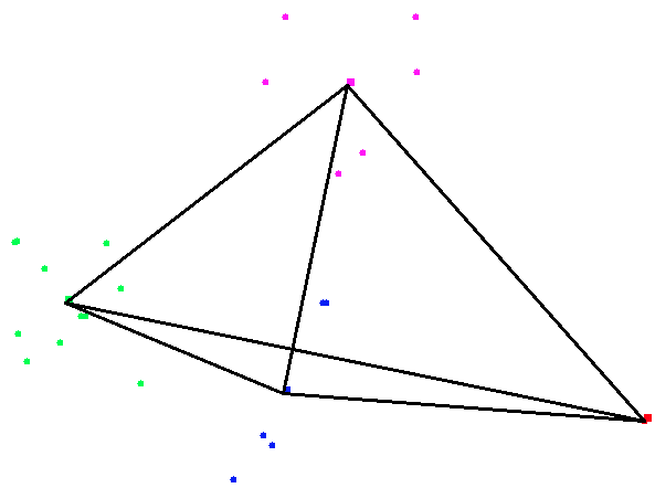
In order to see the final product of your k_means
you will need to call the supplied function
create_cluster_image with a graph_edge_list representation,
a list of initial centroids, and a list of coordinates.
It will use your function to create a clustering of graph, and then
color and print the graph using the OCaml Graphics
module. Here is one such example:
create_cluster_image
          (4, [(0, 1, 1.); (0, 2, 1.); (1, 2, 1.); (1, 3, 1.); (2, 3, 1.); (3, 0, 1.)])
            [(0, (56., -134.)); (1, (61., -151.)); (2, (63., -156.)); (3, (66., -160.))]
              (load_city_coordinates "shortlist.txt")
Which produces the following image: