Your task in this part is to write a simple function apprev
that takes two lists, reverses each and appends them in reverse order.
For example:
apprev [1;3] [5;2] = [2;5;3;1]
rev and append and use these
to write the apprev function.
rev: 'a list -> 'a list
append: 'a list -> 'a list -> 'a list
apprev: 'a list -> 'a list -> 'a list
You are not allowed to use any functions from the List module in this part, but the cons operator (::) is allowed.
To submit: part1.ml and your proofs either as induction.txt or induction.pdf.
For the first part of the assignment, you will be implementing some algorithms on graphs. A Graph is a structure consisting of a set of vertices, V, and a set of edges, E. An edge e is a set of triples (u, v, w) where u and v are the vertices that are connected by e and w is the weight of e. A graph is directed if we treat the edges as pointing from one vertex to another, rather than just connecting them. We will be examining several algorithms that operate on directed and undirected graphs.
In this assignment, we will be using two different representations of
graphs, depending on which is a natural fit for the algorithm in question. The
first is very similar to the adjacency list representation you have probably
already seen. For each vertex, we store a tuple of the vertex and a list of
edges pointing out of that edge. That is all tuples
of the form:
(v, [(v, u_1, w_1); ... ;(v, u_n, w_n)]).
Alternatively, we can use the same representation, but store incoming edges
instead of outgoing edges, so we would have the list of all tuples of the form:
(v, [(u_1, v, w_1); ... ;(u_n, v, w_n)]).
We note that if there are n vertices in the graph, we represent them as
integers from 0 to n-1.
The second representation we will be using stores the number of vertices in
the graph, and holds a single list of all the directed edges. A graph with the
vertex set: {0, ..., n-1} and edge set E consisting of
k edges is represented by the tuple:
(n, [e_1; ... ;e_k])
It will behoove you to use the appropriate representation for the algorithms you will be asked to implement. Functions for converting between the two representations are provided for you to use.
There are no graphs with a "mixed" representation. For any graph, either all vertices have outgoing edge lists, or all vertices have incoming edge lists.
Given a graph G, suppose we would like to give an ordering such that each vertex comes before all the vertices that it has an outgoing edge to. Such an ordering is useful for resolving dependencies, for instance in a compiler, where vertices would be source files and an edge points from u to v if v depends on u.
The algorithm to create such an ordering is quite simple. Each iteration of the algorithm removes one vertex that has no incoming edges from the graph and appends it to the topological ordering. Once a vertex has been removed, the edges originating from it are removed from the graph as well. After this, new vertices with no incoming edges may exist, so we need to continue removing vertices until the graph is empty and we have a topological ordering. If all of the vertices have an incoming edge, this means that the graph has a cycle, and cannot be topologically sorted. Your code should raise an exception in this case.
Another natural object related to graphs that we would like to study is a path between two vertices. If we start at some vertex u, and we can travel along some list of edges and arrive at v, then that list of edges is called a path from u to v. The length of the path is simply the sum of the weights of all the edges. We would like to be able to compute the shortest such path between any two vertices. This has myriad applications, the most obvious being navigation. If we represent locations as vertices and roads between them as edges, with the weight equalling the time it takes to traverse that edge. The fastest way to get from location A to location B would then be the shortest path from vertex A to vertex B. Fortunately, there is an algorithm called Dijkstra's Algorithm which can find exactly this path, as long as it exists and none of the edge weights are negative.
Dijkstra's algorithm is a greedy algorithm, that is it reasons that we can get the overall best result by following the best possible course of action at each step.
The algorithm maintains a shortest path to each vertex, and follows the shortest edges it can, whilst updating the shortest paths to the vertices if it finds an improvement. Initially, the shortest paths are 0 to the initial vertex of the path we are trying to find and infinite for the rest. When the algorithm processes a vertex, (starting with the initial vertex) it checks if the new path to each of its neighbors is shorter than the one currently stored for it. That is, if the best path to the vertex being processed plus the edge weight to one of its neighbors is less than the current best path to the neighbor, we update the neighbor's best path to that edge appended to the best path to the current vertex.
Once we have done this check for each neighbor, we consider the vertex processed, and do not attempt to visit it again or check paths to it, because any subsequent path that comes back to it will form a cycle, which will only increase the path length. We then process the next closest vertex to the initial vertex as dictated by our current understanding of the shortest path to each vertex. The algorithm terminates when we have processed the target vertex, and we return the shortest path to that vertex. Intuitively, we are constantly considering the shortest possible path we could take to each position until we have covered the whole graph or reached the destination.
If the algorithm has run out of vertices to explore and still has not found a path from u to v, no such path exists. Raise an exception to indicate this.
For further explanation, Wikipedia has a good entry on Dijkstra's algorithm.
We can extend our definition of graphs to also admit something called a coloring of the vertices. All this entails is assigning a color to each vertex with the condition that no two vertices connected by an edge share a color. One natural application of such a coloring is coloring in a political map. If we view countries as vertices and put an edge between two countries if they share a border, then we can color the map such that no bordering countries have the same color by assigning a coloring to this graph.
Unfortunately, there is no known fast general solution for coloring arbitrary graphs with a minimal number of colors. For this part of the assignment, you will have to write a verifier that, given a graph and a coloring, returns true if the coloring is valid or false if it is not. You will also have to write a function that produces some k-coloring (that is, uses at most k colors) given a graph or none if it is impossible.
You will be implementing the algorithms described above. In the file graph.ml implement the following methods:
topological_sort: graph -> vertex list
dijkstra: graph -> path
color_verify: graph -> coloring -> bool
color_produce: graph -> int -> coloring option
When testing, we guarantee that the graphs given as inputs to these functions will have the following representation:
For any coloring we test color_verify on, you are guaranteed that every vertex in the graph has a color, and that every vertex specified in the coloring exists in the graph. You do not need to handle nonsensical colorings (colorings that specify vertices not in the graph, or colorings with missing vertices).
The types are fleshed out and explained more thoroughly in the source code and interface (.mli) files.
In general our objective in this part will be to take a list of coordinates and then partition all the coordinates into clusters. We want to then color these clusters and output them graphically.
K-means is an iterative algorithm used in machine learning to partition a set of observations into k clusters. In this case, our observations are coordinates of points. Each cluster is described by a centroid, which is itself just another set of coordinates. A point will belong to a cluster if the centroid of that cluster is closer to it than to any other centroid (as defined by Euclidean distance). At a high level, the algorithm begins with some initial set of k centroids and updates the centroids at each iteration, eventually producing the clustering given by the final centroids.
Given an initial list of centroids, and a list of coordinates, we want to partition all of these points into a list of clusters.
The k-means algorithm follows two key steps:
Keep in mind that in this step, if you have a cluster with no coordinates assigned to it, you will end up dividing by zero when calculating the cluster's new centroid. You should raise an EmptyCluster exception in these cases.
These two steps then repeat until the algorithm converges. We say the algorithm has converged when the assignments to each cluster no longer change.
k_means following the algorithm
described above.
k_means: centroid list -> coordinate list -> cluster list
create_cluster_image. This function takes a
list of centroids and coordinates, as well as a graph_edge_list (one
of the graph representations you saw in Part 1) which will represent
how centroids are connected to each other. Your goal is to partition
all the given coordinates into clusters and then assign a color (where colors
are represented as ints, just as in Part 1) to each cluster such that no
two adjacent clusters (i.e. two clusters with adjacent centroids) have
the same color. You should then call draw_clusters with the necessary
arguments. We have provided you with this function, which uses the OCaml
Graphics
library to display an image with your colored clusters and centroids.
draw_clusters is the only function you are allowed to call
that uses side effects.
create_cluster_image: Graph.graph_edge_list -> centroid list -> coordinate list
    -> unit
All of the types necessary to complete this part are more thoroughly explained in the source code (cluster.ml).
To submit: cluster.ml
You will build a custom toplevel containing all of your PS3 code. We have
provided you with a script called buildToplevel.bat (or buildToplevel.sh for
Unix) which creates such a toplevel. To start the toplevel, execute the script
runToplevel.bat (or runToplevel.sh). The Graph and
Cluster modules will be automatically loaded. However, the modules
are not opened, so you will still have to type open Graph;;
or open Cluster;;.
You will find that we have provided you with two text files, "shortlist.txt" and "longlist.txt". These have the coordinates to several US cities.
In order to see the final product of your code you will need to callcreate_cluster_image with a graph_edge_list representation,
a list of initial centroids, and a list of coordinates. Here is one
such example:
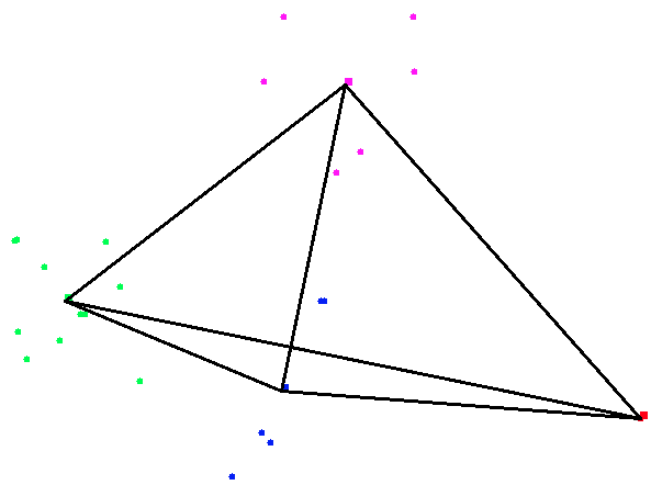
create_cluster_image
          (4, [(0, 1, 1.); (0, 2, 1.); (1, 2, 1.); (1, 3, 1.); (2, 3, 1.); (3, 0, 1.)])
            [(0, (56., -134.)); (1, (61., -151.)); (2, (63., -156.)); (3, (66., -160.))]
              (load_city_coordinates "shortlist.txt")
The result of this produces the following image: