
For the first part of the assignment, you will be implementing some algorithms on graphs. A Graph is a structure consisting of a set of vertices, V, and a set of edges, E. An edge e is a set of triples (u, v, w) where u and v are the vertices that are connected by e and w is the weight of e. A graph is directed if we treat the edges as pointing from one vertex to another, rather than just connecting them. We will be examining several algorithms that operate on directed and undirected graphs.
In this assignment, we will be using two different representations of graphs,
depending on which is a natural fit for the algorithm in question. The first is
very similar to the adjacency list representation you have probably already
seen. For each vertex, we store a tuple of the vertex and a list of edges
pointing out of that edge. That is all tuples of the form:
(v, [(v, u_1, w_1); ... ;(v, u_n, w_n)]).
Alternatively, we can use the same representation, but store incoming
edges instead of outgoing edges, so we would have the list of all tuples
of the form:
(v, [(u_1, v, w_1); ... ;(u_n, v, w_n)]).
We note that if there are n vertices in the graph, we represent them
as integers from 0 to n-1.
The second representation we will be using stores the number of vertices in the
graph, and holds a single list of all the directed edges. A
graph with the vertex set:
{0, ..., n-1} and edge set E consisting of k edges is
represented by the tuple:(n, [e_1; ... ;e_k])
Given a graph G, suppose we would like to give an ordering such that each vertex comes before all the vertices that it has an outgoing edge to. Such an ordering is useful for resolving dependencies, for instance in a compiler, where vertices would be source files and an edge points from u to v if v depends on u.
The algorithm to create such an ordering is quite simple. Each iteration of the algorithm removes one vertex that has no incoming edges from the graph and appends it to the topological ordering. Once a vertex has been removed, the edges originating from it are removed from the graph as well. After this, new vertices with no incoming edges may exist, so we need to continue removing vertices until the graph is empty and we have a topological ordering. If all of the vertices have an incoming edge, this means that the graph has a cycle, and cannot be topologically sorted. Your code should raise an exception in this case.
Another natural object related to graphs that we would like to study is a path between two vertices. If we start at some vertex u, and we can travel along some list of edges and arrive at v, then that list of edges is called a path from u to v. The length of the path is simply the sum of the weights of all the edges. We would like to be able to compute the shortest such path between any two vertices. This has myriad applications, the most obvious being navigation. If we represent locations as vertices and roads between them as edges, with the weight equalling the time it takes to traverse that edge. The fastest way to get from location A to location B would then be the shortest path from vertex A to vertex B. Fortunately, there is an algorithm called Dijkstra's Algorithm which can find exactly this path, as long as it exists and none of the edge weights are negative.
Dijkstra's algorithm is a greedy algorithm, that is it reasons that we can get the overall best result by following the best possible course of action at each step.
The algorithm maintains a shortest path to each vertex, and follows the shortest edges it can, whilst updating the shortest paths to the vertices if it finds an improvement. Initially, the shortest paths are 0 to the initial vertex of the path we are trying to find and infinite for the rest. When the algorithm processes a vertex, (starting with the initial vertex) it checks if the new path to each of its neighbors is shorter than the one currently stored for it. That is, if the best path to the vertex being processed plus the edge weight to one of its neighbors is less than the current best path to the neighbor, we update the neighbors best path to that edge appended to the best path to the current vertex.
Once we have done this check for each neighbor, we consider the vertex processed, and do not attempt to visit it again or check paths to it, because any subsequent path that comes back to it will form a cycle, which will only increase the path length. We then process the next closest vertex to the initial vertex as dictated by our current understanding of the shortest path to each vertex. The algorithm terminates when we have processed the target vertex, and we return the shortest path to that vertex. Intuitively, we are constantly considering the shortest possible path we could take to each position until we have covered the whole graph or reached the destination.
A Minimum Spanning Tree of a graph is the subgraph with the lowest-weight subset of edges such that each node is connected to every other node. This property is defined for undirected graphs, so we shall consider our edges to point in both directions for the following discussion. If there are some vertices that are unconnected, then we would like to find the minimal collection that spans each connected component. We can represent these spanning trees of connected components elegantly and efficiently in something called a disjoint set forest, an implementation of which is provided for you.
An algorithm that achieves this is another greedy algorithm called Kruskal's algorithm. The algorithm works by starting with a graph of all the vertices isolated, that is each vertex is its own connected component. It then forms the ascending ordering by edge weight of all of the edges in the original graph. The algorithm then processes each edge in this order, adding it in only if it connects two previously unconnected components. Once we have processed all of the edges, the resulting graph is a minimum spanning tree, or a forest of minimum spanning trees of the connected components.
We can extend our definition of graphs to also admit something called a coloring of the vertices. All this entails is assigning a color to each vertex with the condition that no two vertices connected by an edge share a color. One natural application of such a coloring is coloring in a political map. If we view countries as vertices and put an edge between to countries if they share a border, then we can color the map such that no bordering countries have the same color by assigning a coloring to this graph.
Unfortunately, there is no known fast general solution for coloring arbitrary graphs with a minimal number of colors, so we will have to settle for another greedy algorithm. Unlike the ones in the previous sections, this algorithm is not optimal. The way the algorithm works is it goes through the vertices in increasing order of degree and colors them one at a time, taking care to only use new colors when it has to. That is, we process a vertex by checking whether any of the colors we have already used so far is consistent with the current coloring of the graph. If none of the existing colors work, we introduce a new color and color the vertex with that. Otherwise, we simply pick one of the previously used colors that works and move on to the next vertex.
topological_sort: graph -> vertex list dijkstra: graph -> path kruskal: graph -> DisjointSet.universe color_graph: graph -> coloring |
|
sigma = 0.5, k = 500,
and min_size = 50.
The goal of image segmentation is to partition an image into a set of perceptually important regions (sets of contiguous pixels). It's difficult to say precisely what makes a region "perceptually important", and in different contexts it could mean different things. The algorithm you are going to implement uses the variation in pixel intensity as a way to distinguish perceptually important regions (also called segments). This criterion seems to capture our intuitive notion of a segmentation quite well.
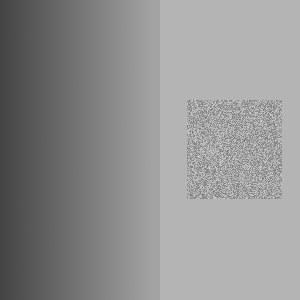
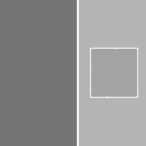
To illustrate how the algorithm uses intensity variation as a way to segment an image, consider the grayscale image below. The image on the right is the result you get from segmenting the image on the left. Each segment is given a white outline and given a solid color. All of the pixels in the large rectangular region on the right have the same intensity, so they are segmented together. The rectangular region on the left is considered its own segment because it is generally darker than the region on the right, and there is not much variation between the intensity of adjacent pixels. Interestingly, the noisy square on the right is considered a single region, because the intensity varies so much.
There are some large differences between the intensities of adjacent pixels in the small square region; larger even than the difference between pixels at the border of the two large rectangular regions. This tells us that we need more information than just the difference in intensity between neighboring pixels in order to segment an image.
Note that the algorithm found a few thin regions in the middle of the image. There is no good theoretical reason why these regions should be there: they were simply introduced as an artifact of smoothing the image, a process that will be discussed later.
 |
 |
Parameters: sigma = 0.5, k = 500, min_size = 50.
Image segmentation provides you with a higher-level representation of the image. Often it is easier to analyze image segments than it is to analyze an image at the pixel level. For example, in the 2007 DARPA Urban Challenge, Cornell's vehicle detected road lines using this image segmentation algorithm. First, a camera in the front of the car takes a picture. Then the image is segmented using the algorithm you are going to implement. Since road lines look quite different from the road around them, they often appear as distinct segments. Each segment is then individually scored on how closely it resembles a road line, using a different algorithm.
Consider the image as a graph where each pixel corresponds to a
vertex. The vertex corresponding to each pixel is adjacent to the
eight vertices corresponding to the eight pixels surrounding it (and
no other vertices). Each edge has a weight, w(v1,
v2), defined to be
 where ri,
gi, bi are the red, green, and blue components
of pixel i respectively.
where ri,
gi, bi are the red, green, and blue components
of pixel i respectively.
The image segmentation algorithm works by building a graph that contains a subset of these edges. We will start with a graph that contains all of the vertices but no edges. For each weighted edge, we will decide whether to add it to the graph or to omit it. At the end of this process, the connected components of the graph are taken to be the segments in the image segmentation (so we will refer to segments and connected components interchangeably).
We define the internal difference of a
connected component C to be  where
where E(C) is the
set of edges that have been added to the graph between vertices in
C, and w(e) is the weight of e.
If C contains no edges, then define Int(C) =
0.
Also define T(C) = k/|C|, where k is some
fixed constant and |C| is the number of vertices in C.
We call this the threshold of C.
At the beginning of the algorithm, there are no edges, so each
vertex is its own connected component. So if the image
is w by h pixels, there are
w*h connected components. Sort the edges in
increasing order. Now consider each edge
{v1, v2} in order from
least to greatest weight. Let C1
and C2 be the connected components that
vertices v1 and v2 belong to respectively.
If C1 = C2, then omit the edge.
Otherwise, add the edge if
w(v1, v2) ≤ min(Int(C1) +
T(C1), Int(C2) + T(C2)).
This merges C1
and C2 into a single component.
Note that T(C) decreases rapidly as the size
of C increases. For small
components, Int(C) is small (in fact, it is 0
when |C| = 1). Thus Int(C) + T(C) is
dominated by T(C) (the threshold) when C
is small and then by Int(C) (the internal difference)
when C is large. This reflects the fact that the
threshold is most important for small components. As we learn more
about the distribution of intensities in a particular component
(information that is captured by Int(C)), the threshold
becomes less important.
Once you have made a decision for each edge in the graph, take each connected component to be a distinct segment of the image.
You will find that the above algorithm produces a number of tiny,
unnecessary segments. You should remove these segments once the
algorithm is finished by joining small connected components with
neighboring components. Specifically: order the edges that were
omitted by the algorithm in increasing order. For each edge, if the
components it joins are different, and one or both has size less
than min_size, then add that edge to the graph.
Call min_size the merging constant.
Before segmenting an image, you should smooth it using a Gaussian filter. Smoothing the image makes it less noisy and removes digitization artifacts, which improves segmentation. We have provided you with the code to do this, so you do not need to implement it yourself. Gaussian smoothing takes a parameter σ. The value σ = 0.8 seems to work well for this algorithm; larger values of σ smooth the image more.
We have provided you with a module called Image,
which provides functions for manipulating images. The module
contains functions for loading and saving bitmap files,
Gaussian smoothing, and a function for displaying images using
the OCaml Graphics
library.
Please implement the image segmentation algorithm described
above in the Segmentation module as three
separate functions: segment_graph,
segment_image, and
merge_small_segments.
segment_graph should take an arbitrary graph
represented as a size and list of weighted edges
as input and segment it using the above
algorithm (it should not matter that the graph does not correspond
to an image). This function should return a value of type
segmentation. You are free to define
segmentation however you like. However, we will still
need to test your code. Thus you should write a function
segments which takes a graph and a segmentation and
returns a list of components (i.e. segments). Each component will be
represented as a list of the integers corresponding to the vertices
in the component.
merge_small_segments should take a
segmentation, a list of edges, and a merging threshold
min_size. It should merge segments whose size is less
than min_size as described above. Again, we will test
this function using the segments function.
segment_image should take an image as input and
return a segmentation that partitions the pixels in the
image into segments. As discussed above, you should smooth the image
first (using Image.smooth), then build a grid graph and
segment it using segment_graph and merge small segments
using merge_small_segments.
segment_image should have complexity O(nlog(n))
where n is the number of pixels in the image. Choose your data
structures carefully to achieve this runtime. You may write
imperative code for this assignment.
color_segments should take an image and its
segmentation as input and return an image where the segments are
outlined and colored, like the one at the top of this writeup. You
should color any pixel that is adjacent to a pixel from a different
segment (using the 8-neighbor definition for adjacency described
above). Then for each segment, compute the average color of all of
the pixels in that segment (i.e. by separately computing the average
red, green, and blue components of the colors in that segment), and
assign this color to every pixel that is not a border pixel. Segmentation.segment_and_show that segments a bitmap
file, colors it using color_segments, shows you the
result, and saves the result as segmented.bmp.
Note: The results of your algorithm may be slightly
different from the examples given here, because the order that you
consider the equal-weight edges influences the segmentation. In
other words, after you sort your edges by weight, if you then
permute the edges with equal weight, you may get different
results.
To submit: segmentation.ml.
You will build a custom toplevel containing all of your PS4
code. We have provided a script called buildToplevel.bat (or
buildToplevel.sh for Unix) which creates such a toplevel. To start the
toplevel, execute the script runToplevel.bat (or runToplevel.sh). The
Image and Segmentation modules will
automatically be loaded.
If you would like to define additional modules, please put them in segmentation.ml. This will make it easier to test your code.
Any functions or modules defined in segmentation.ml will be
available in the Segmentation module. For example, if
you define a module named Foo in segmentation.ml,
it will be known as Segmentation.Foo.
This phenomenon occurs because when you compile OCaml code using
ocamlc, each file you compile automatically defines a module. For
example, functions defined in foo.ml are automatically placed
into a module called Foo without using the module Foo
= construct.
A tree is a connected graph with no cycles in it. Equivalently, it is a connected graph with exactly N-1 edges, where N is the number of nodes. The diameter of a tree is the maximum distance between some pair of two nodes. It turns out that there is a simple algorithm for finding the diameter of a tree: