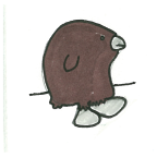
Swamp_Slime	Shy_Frecklepuss	Fuzzy_Trible	Gray_Floop	Ballards_Protoduck

A few of the 40 animals in the CS2110 bestiary.  Credit for the pictures goes to our talented artistic consultant, Ursula Hilsdorf. 

Note: This page gives an overview of the entire 5-part assignment.  Below you'll find links that will take you to the detailed versions of each of the five assignments.  You'll use CMS to hand in your solutions.

1. Link for Assignment one: Due Sept. 9 at 11:59pm

2. Link for Assignment two: Due Sept 22 at 11:59pm

3. Link for Assignment three: Due Oct 9 at 11:59pm

4. Link for Assignment four, Due Nov 8 at 11:59pm

5. Link for Assignment five, Due Dec 3 at 11:59pm.  Whew!

Creating an Evolutionary Tree

During fall of 2009, CS2110 students will be working on a semester-long project that has a series of intermediate deliverables.  Even before explaining what this project is about we want to reiterate that  for assignment 1, each student is expected to work on his or her own, and for other assignments you can work in teams of 2, but no more, and teams can't collaborate with other teams!  You are welcome to have non-specific dialog about the project with friends or a study group, but every line of code you type needs to be written by you personally, or by you and your teammate on A2-A5, and you can’t show other people your solutions before the deadline for handing them in.  (Suggestion: read the section on “automated cheating detection.)

One small comment: The assignment is designed to be solvable by a person working by his or herself.  We allow teams on A2-A5 but aren't really encouraging or assuming that you'll work in teams.  In fact it is better for you to work on your own, just as a running who trains by jumping in the team car for half of each workout probably won't end up being as strong as a runner who runs the full distance on her own!

What You’ll Do

The goal of the project is to use genome data to figure out the relationship between a set of animals.  We’ll provide pictures of the animals and some other data, and as part of that data we'll give you the animal's DNA.  Using code we develop during the semester, we’ll tackle problems such as extracting genes from the DNA, comparing to see how similar two genes are, and finally building a graph (a tree) representing the evolutionary history of the creatures and displaying the data in web pages.  The problem is a simplification of one of the most important problems seen in modern biology. 

Genomic computations in “reality” can be fairly messy, so for CS2110 we’ll be using a somewhat simplified genetic model.  The simpler version isn’t completely realistic, but it does parallel the actual computational biology problem, while limiting itself to technical ideas that are at the right level for students taking a second semester Java course.  We’re hoping that you’ll discover that without learning a huge amount of computer science, you can already do some really amazing things.  We also want to see you get experience writing high-quality code – this is a skill you can only learn by doing. 

Our semester-long project will be broken into five separate sub-projects, each linked to material we’ll be learning in lecture.   Each subproject will involve implementing some set of Java classes that supports a specific interface that we’ll define carefully.  (One warning: Even if you think the interface we request is lame, you still need to use it because our automated testing program checks for it!)  When practical, we’ll provide a very limited test setup that you can use to make sure that your solution does match what we expect, but then when you hand in your solution, we’ll test it against a harder set of scenarios.   So your job is to write code that definitely works in our simple tests, but in fact that can also work for cases that it hasn’t previously “encountered”.  This may mean that you need to develop your own tests beyond the ones in our limited testing setup, to make sure that coverage is adequate!

To get full credit, each assignment that you hand in needs to be well-written, properly debugged code that correctly implements the functionality and interface we assigned, and needs to run on our full range of automated test scenarios. Your code has to be properly commented and clear, with good choices of variable names and if something can be done in a simple way, or in a complicated way, our graders will deduct points for overly complex solutions.  (The famous phrase is KISS: Keep it Simple, Stupid!)  All our projects have reasonably simple solutions.

As a safety net, after each subproject is handed in, we’ll release Professor Birman’s solution for that same problem.  This way, you can tackle the next subproject even if yours had serious bugs. Just the same, we really would encourage you to work with your own code.  It will not be possible to get top grades in CS2110 unless you use your own code entirely, or at least as much as possible.

The Project

As you know from your biology classes, each species is defined by a unique genome: a sequence of amino acids from a small alphabet.  The real genome is composed of triples (so-called “codons”) of letters representing the associated amino acids: A, C, U and G.   In CS2110, we won’t worry about codons, and will work with a fake genomic alphabet with amino-acid symbols A, C, I and O. 

The genome mixes junk (“non-coding”) DNA) with genes that encode the proteins that make up the animals and control them.   Our CS2110 DNA is like this too.  In our DNA sequences, a gene always starts with a special three-letter code: AOC, and ends with a second three-letter code: ICA.  Thus, DNA sequence AOACOAOCOICCACOIIICOCIOICAIIOO actually consists of a single gene and some junk: AOACO start OICCACOIIICOCIO end IIOO.  The AOACO and IIOO parts are examples of junk DNA, whereas OICCACOIIICOCIO is an example of a gene.  Notice that the start and end sequence aren’t included in the gene itself – they are like another form of junk.

Human genes are billions of amino acids long.  CS2110 genes are a little shorter: a typical DNA sequence will be about 50,000 letters in length and might contain as few as 10 or as many as 50 genes, each of which would be 150 to 500 letters long.    Note:  the longest DNA sequence in our experiments will never be more than 99,999 letters long.  The longest gene will never be more than 999 letters long.

When a species reproduces, its genes change in many ways.  Even within a single species there can be small DNA differences in the genes carried by individuals, and each child inherts some genes from each of its parents.  But a new species can arise when gene copying mistakes occur during cellular reproduction.   For CS2110, we’ll focus on genes that arise by duplication (e.g. an entire gene or set of genes is simply copied twice from the parent to child), swaps (some short sequence of letters is swapped with some adjacent sequence), insertions (of small numbers of letters) or deletions.

For example, let’s look a closer look at our sample gene from above, call it G1 :  "OICCACOIIICOCIO”.  (We underlined two letters to draw your attention to them).  Now suppose that we were shown a gene G2 : "OICCCAOIIICOCIO”.   A possible relationship is that G2 could have originally been the same as G1, but then a two-letter swap occurred (AC became CA).  Of course there are also other ways this could have happened.  For example, perhaps the A was deleted in the first gene to create a gene G’, and then later an A was inserted right after the C to create G2.  In fact all sorts of crazy things could have happened… with these simple rules there are infinitely many ways that G1 could have become G2.  The swap shown is just the most likely explanation – the shortest explanation.

For CS2110, we’ll be developing a gene comparison procedure that wouldn’t work for humans (where gene comparison is a very complex question), but does work for our « fake » genomic data because the genes were actually created synthetically and designed to be relatively easy to compare.  We’ll be using a method inspired by a real gene comparison algorithms (examples of famous ones are Smith-Wasserman and BLAST – look them up in Wikipedia if you get interested in the topic).

The basic idea is to define a distance metric with which we can score gene similarity.  To make things simple, isuppose that when two genes are directly related, the changes all occur at one part of the sequence.  Thus if G1 evolved into G2, we can rewrite G1 = abc and G2 = adc, and all the changes will have occurred in the region that used to contain  b and now contains d.

Given G1 = abcand G2 = adc, such that G1 comes before G2 under the rules defined in assignment two, we’ll define a distance score this way:

1.       Count all the letters in b and all the letters in d.  For example, perhaps b contains 3 A’s, 2 C’s, 2 I’s and 5 O’s.  Now do the same for d: maybe you’ll find 0 A’s, 1 C’s, 5 I’s and 9 O’s. 

2.       Sum up letters in both strings: 1 C, 2 I’s and 5 O’s for a total of 8.  We’ll score these as 15 points each: 120 points.  Below we use the constant "SCost" for this: "same characters but in some sort of different order".

3.       Next compute the letters in one string but not the other.  We’ll score these as 8 points if the characters are found in both strings, but the number of instances differs (DCost), and 25 points if one string contains a character that the other string doesn't contain at all (DDCost).  In our example: both strings contain the characters C and I and O, so we get (1+3+4)*DCost = 64 but only one string contains A's: 3*DDCost = 75, giving a total of 139.

Of course we oversimplified: changes could occur at a few places, not necessarily all in one region.  Our "real" solution needs to take this into account.  Given two genes, we'll start by computing the length of any prefix they have in common, e.g. XYZ <stuff> and XYZ <stuff'>.  Next, we'll look for suffixes they have in common: <stuff> XYZ and <stuff'> XYZ.  So now we're down to <stuff> and <stuff'>, which (if they aren't null strings) differ at least in the first and last characters, but could contain a "section" that matches.

Let's assume that if <stuff> and <stuff'> are of different lengths, then <stuff> is the shorter of the two.  We'll take a "window" of MinMatch characters (4, as defined below) within <stuff> and "slide" it along <stuff'> looking for a match.  For example, if <stuff> was ACIOCAO and <stuff'> was CIAACIOCCC, then we can slide ACIO (the first 4 characters of <stuff>) along <stuff'>: first we would check it against CIAA, then IAAC, then AACI and then (horray!) ACIO.  Assignment two explains exactly how this needs to be done; use the detailed explanation in the assignment when coding a solution.

If we find a match, we can "grow" that match one character at a time towards the right: the longest match possible is ACIOC.  So now we know that <stuff> should really be fragmented into three parts: a null string, then ACIOC, then AO.  And <stuff'> into three parts too: CIA, then the matching section, ACIOC, and then the remainder, CC.  We use our difference computation on the first pieces: a null string versus CIA. (Score 3*DDCost = 75)  We have an exact match for ACIOC.  And then we repeat this whole procedure for the remainder: <stuff> will now be AO and <stuff'> will be CC.  These are shorter than MinMatch, so we're finished and we compute the difference computation on AO and CC (score 4*DDCost = 100), adding that to the running total.  Our two genes are at distance 175 from each other.

Notice that had we not used this fancier scheme, we would have gotten a completely different answer and, worse, that answer would treat a matching section (ACIOC) as if it differed between the two.   

Here are some constants we'll use for the sorts of comparisons just described (and for some additional ones mentioned below):

public class Constants {
            public static final int SCost = 15; // Gene: Cost for same characters in different order
            public static final int DSCost = 8; // Gene: Cost for different counts but of the same characters
            public static final int DDCost = 25; // Gene: Cost for completely different characters
            public static final int MinMatch = 4; // Gene: When looking for strings of the form <stuff> XYZ.... and <stuff'> XYZ, XYZ must be at least MinMatch long
}

This scoring function is what we would call a “heuristic” – a rule of thumb that will suffice for our purposes in CS2110.   It may seem a bit ad-hoc, but in fact the Smith-Wasserman and BLAST algorithms also use heuristics, and of a very similar nature.  The problem is that computing the exact way that G1 evolved into G2 is such a hard problem – there are too many possibilities to explore, and in general, more than one might lead to the right place.  Worse, we can’t really know that evolution followed the shortest path.  So this is a case in which there isn’t any way to know the “true” answer. A good rule of thumb may be about as good as we can do!

You will find that when genes are reasonably similar, the scoring function tends to be 750 or less (often much less).  When genes are very different the score rises sharply.  In fact we'll limit the maximum difference to CommonCutoff: 2500 in our table of constants.

What about comparing entire animals?  We can do this using a second kind of scoring function to compute an animal’s closest relative.  For example, perhaps cats have 73 genes in their genome and dogs have 81, and out of these, 45 are common to the two.  We’ll use our gene comparison functions to try and measure the distance from dogs to cats.  If the two are very closely related we would expect that all the different genes are actually pretty closely related.  In contrast, if we find huge differences, that would suggest that dogs and cats are pretty distant from each other in an evolutionary sense.   Of course, keep in mind that our little zoo is just a sample of all the animals that ever existed – dogs and cats could be pretty closely related, but there could be many other animals between their common ancestor and each species.  So here’s the scoring function we’ll use:

Given animal A with genes {A₁, …. A_k} and animal B with genes {B₁, … B_n}

1. For each gene in A, find the closest gene in B.  Add the distance to score.   [Note: HW4 will slightly modify this rule]

2. For each gene in B, find the closest gene in A.  Add the distance to score.  [Note: HW4 will slightly modify this rule]

3. Divide score by two; this is the "animal to animal" distance.

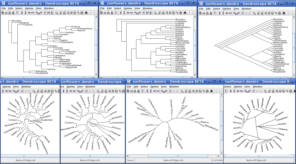
This can be used to compute a matrix of Animal-to-Animal "distances".  Given that matrix, we can now compute what is called a Phylogeny tree: we take an animal that is believed to be the most primitive ancestor in the group, and then look for an animal in our bestiary that is as similar as we can find to the root animal.  We attach this best matching animal below our root.  Now we repeat the process, looking for the animal that represents the closest match to any animal already in the tree, and again attaching it as a child of the animal with which the match was closest.  And we continue until we've put every animal below its best matching relative.  (Notice that you end up with a very different tree if you start with a different first choice -- the "root" matters!)

Each CS2110 project will come with its own assignment handout, but here’s a high-level overview of the projects and a short description of what each one entails.

Project 1:  We’ll start by writing Java classes to just read in the basic genomic data for our menagerie of animals.  Each animal will be defined by a file that contains the animal’s English-language name, its Latin species name, a filename where a picture of the animal can be found and its DNA sequence.   Most of these DNA sequences are long and we do not recommend printing the full set of files.  However, we will have some « fake » animals with very short DNA sequences that you can work with for testing, and those can be printed if necessary.  The files to read will be provided as arguments to your program.  (Use the Eclipse "run configurations" page to set these runtime arguments and also to tell Eclipse what folder to launch your program in -- obviously, that should be the folder in which the data files are located.  You can create multiple configurations and give them each different names, which is convenient for testing).

1. As you read each file, you’ll « parse » the contents to break out the different pieces of information contained within it.  You’ll use this to construct an object representing each animal.

2. Rather than storing the entire DNA string, which may have a lot of junk, you’ll break the DNA string up into its constituent set of genes.

3. Store each gene into a special Java structure called a Hashmap that we’ll learn about in class, using the gene string itself as a hash key.  This will let you create a set of the entire set of genes found in our entire menagerie of animals. Assign each unique gene a number and use these to generate gene names: G1, G2, etc.  The idea is this: if the program sees a new gene (one not already in the gene map) it assigns it a new name like the ones above.  If an animal has a gene that has shown up previously, we’ll use the same name for that gene.  Thus each separate gene name corresponds to a genetic code that differs from every previously known gene code.

1.  We’ll modify our project 1 code so that the gene numbers actually respect a sorting order.  This order will list shorter genes before longer ones, and break ties alphabetically.  Thus, G1 would necessarily either be shorter than G2, or be the same length but alphabetically smaller than G2. 

2. We’ll also start to work on a gene comparison algorithm that computes an estimate of the evolutionary distance between two genes.   Doing a good job of designing the gene comparison class is important, so we’ll do this carefully, providing a number of methods that you can use later in subsequent stages of the project. One of the tricky aspects will be the problem of breaking up two differing genes into sequences of the form we showed above (abc).  What makes things complicated is that this three-sequence example makes it seem as if every pair of genes really has a single region where differences occur.  In fact two genes might have multiple sections that are similar and more than one region with differences, and our solution will take this into account.    We'll do this using the procedure described earlier, in which we look for a section of length MinMatch or longer that matches and then extend it, in this way carving off sections that differ and then skipping matching sections, and then repeating the process if there are more differences.

3. We’ll use the gene comparison class and will use it to compute an all-to-all matrix of relationships between all the genes in our entire data set (computed in project 1).  This will let us list, for each gene, the gene other than itself that has the most similarity.  For example, G1 is identical to itself, but perhaps is very different from G2.. G47, rather similar to G48, etc.  So G1 might be “most similar” to G48.  G48, on the other hand, might be “most similar” to G19, etc.  You'll use the matrix of gene-to-gene distances later, to speed up Project 3 by avoiding recomputing distances more often than needed.  Notice that if you compare G1 with G7, or G7 with G1, you should get the identical score.  It might be wise to check that your solution does this correctly.

1. First we'll enhance the gene-to-gene comparison table from A2 with a slightly fancier comparison policy that gives more accurate results.  This is explained more carefully in the handout.

2. Next build a second all-to-all matrix giving animal-to-animal comparison scores, using the method described earlier, for each pair of animals.  Our scheme will have the property that A compared to B and B compared to A give the same score.

3. Write a method that, for each animal, looks up its closest relative.

4. Using a Java display interface that we'll explain how to build in the detailed handout, build an interactive user interface that shows animals and their pictures and, when an animal is clicked, highlights the animals most similar to it.  It will do this by redrawing the background color of the selected animal’s picture in a bright color and then recoloring all the other animals with colors that vary based on their distance from the selected one.  It will also display that animal slightly larger on the right and show its closest matching neighbor, and will print their names (see the detailed handout).  There are a total of 40 animals in the data set; we recommend displaying them in four lines of ten animals each line.  However keep in mind that although we could test your application on all 40, we often will use a subset of them.  For example, we might decide to focus on animals A0...A38, or animals with even numbers, or just animals A1 and A2. 

5. For extra credit on assignment 3, add a "slider" with a scale from 0 to 5000.  If the user slides the bar, for example to d, find all "families" of animals such that " Family F, "  Animal A,B Î F, AnimalDist(A,B) < d.  Thus if d=1000, we would find some number of families, perhaps 15, such that each family is a set of animals that are all within distance d of every other member of that same family.  Color code each family with a distinct color.  As one slides the slider, dynamically recompute the families and refresh the display accordingly.

A typical input file for Dendroscope would have a name like “Beasts.txt” and would contain a line like this: (A1:0.0097,(A2:0.45,A3:0.717)).  You just tell the program to read in the file from the file « open » command and it generates the tree automatically.  Initially, no animals will be shown, but if you use the « option » that tells the program where to find the image files, it will display their pictures too.  You can also put this information right inside the input file if you like.  Obviously, you’ll need to produce this file from your program, not by hand.

If the input file uses node names like we did above (A1, A2, A3), then  Dendroscope would expect that pictures of the animals are in files named A1.bmp, A2.bmp, etc.   Of course A1 is just a name and you can use anything else : Zebra would work, or Freckleopolous, etc.   One slight issue is that if the names are too similar, Dendroscope sometimes gets confused and puts the wrong picture next to a node -- this is some kind of bug in the application.  If you run into this problem, please contact Professor Birman and he can help -- he's already been down this path.

The floating point numbers tell Dendroscope how long to make the edges in the graph – if you don’t give a number, it uses 1.0 as the default.  Using .0097 for A1 causes it to be displayed « high » in the tree relative to A2 and A3 ; A2 will be below A1 and A3 end up lowest of all.  The program offers many tree representations and you can try different versions, depending on your mood.

Here's an example of a Dendroscope tree displayed in the various display options it offers, but without the little pictures shown (you need to tell it to "load taxon images" if you want to see the images too, and for the figure below, from their user manual, they didn't do so):

For our purposes in CS2110 we'll use the top left tree representation but we'll also have animal names and images associated with the "inner" nodes, whereas in the example on the top left, the inner nodes weren't given names.  We'll need to tell your application which animal should be at the root of the tree (the ancestor of all the animals in it); if you think about the way we build these trees, you get a different tree depending on which animal is put at the root!  (In addition to this, once you have a tree, you can make it look very different by telling Dendroscope to use some other animal as the root node, but this is a different thing -- the tree itself would be the same).

Awesome competition for big prizes!

Assignment 5 will also feature the annual competition to be the best hacker in CS2110!  Here's how it works: When we announce the assignment, it will include an optional special feature that you can tackle if you dare.  Our TAs will look at solutions that work and pick the best solution as the prize winner.  We plan to have awesome prizes in a few categories: best performance, best algorithm, and best code quality.  The race begins on the day we officially release A5!

 Automated Cheating Detection

We’ve noticed that some Cornell classes do a so-so job of enforcing the academic integrity policy.  In CS2110, we have a solution: we’re using an automated system that uses sophisticated artificial intelligence techniques combined with some pretty fancy program analysis tools to notice unusual similarities between programs turned in by different people.  It is important to realize that these tools really work and that they are quite hard to fool.  So while it might seem tempting to borrow a solution from some, change the variable names and comments, or reorder the statements, our tools would be very likely to figure out what you did.   We take cheating seriously, and cheating with an attempt to cover it up is grounds for failing the course outright.  Realistically, it is much easier to just do the assigned problems than to get away with handing in code someone else wrote, because short of rewriting that code completely from scratch, we’ll catch it.

So you’ve been warned:  It is just not possible to get away with cheating in CS2110.  Please do your own work, and come talk to Professor Birman, or the TAs, as often as needed if you get stuck and need help.  We’ll get you back on track.  In contrast, borrowing a solution from a pal will just get both of you into very serious trouble.