Assignment 1
Table of Contents
- 1 Preamble: Setting up Taichi
- 2 First part: Procedural turbulence for flow past an obstacle
- 3 Second part: Mass-spring cloth simulation
- 4 Submission
This assignment explores animations that can be computed using particle systems, and it has two parts. One is a 2D simulation of turbulent flow that uses procedural noise to concoct fake flow fields that look like fluids. The second is a 3D mass-and-spring cloth simulation, which simulates dynamic folding and wrinkling, but doesn’t handle self-collisions in the cloth.
1 Preamble: Setting up Taichi
Install Taichi with pip install taichi and make sure you
are able to run the Julia Fractal.
We recommend using Anaconda to
install Python 3.8, and then using pip to install Taichi
within a conda environment. This will help keep your setup for this
class separate from other Python environments you might need for other
projects. Once you have installed Anaconda you can do this with these
commands:
conda create --name cs5643 python=3.8
conda activate cs5643
pip install taichi pywavefront
Be sure your Taichi version is at least 1.4.
For the starter code, go to our assignment repository at this place and make a fork. Your fork should be a private repository. This will let you easily pull updates related to bug fixes and later assignments from our repository into yours.
Then clone your repository with:
git clone git@github.coecis.cornell.edu:yourNetID/<path to your repo>.git
2 First part: Procedural turbulence for flow past an obstacle
For the first part of this assignment you will implement an animation of particles in a 2D flow field that looks like the flow of a fluid around a circular obstacle. We’ll use the approach known as curl noise, as introduced in Bridson 2007.
The idea of curl noise is to generate divergence-free velocity fields by defining a vector field known as the “potential” and then defining the the velocity field as a derivative of the potential—in particular, the curl of the potential. Because the divergence of the curl of any vector field is zero, this ensures your velocity is divergence-free so that particles will flow around without clumping.
This assignment is in 2D, so the potential is considered to be a vector pointing in the \(+z\) direction, and in the code it can be represented by a scalar field.
In this assignment we will define the potential as the combination of three pieces:
- A “background flow” potential \(c(\mathbf{x})\) that ramps up linearly from bottom to top to define a steady flow from right to left.
- A modulation function \(r(\mathbf{x})\) that passes smoothly through zero at the surface of the obstacle.
- A procedural turbulence function \(n(\mathbf{x})\)
- A turbulence window function \(A(\mathbf{x})\) that is nonzero in the region to the left of the obstacle where we want to see a turbulent wake, and ramps down smoothly to zero outside that region.
The final potential is \(\phi(\mathbf{x}) = r(\mathbf{x})(c(\mathbf{x}) + A(\mathbf{x})n(\mathbf{x}))\).
You may use the starter_code.py to kick-start your
implementation of this part.
2.1 Laminar flow
Start by getting the laminar part of the flow (i.e. without the
noise-based “turbulence”) working. Start with a simple first-order
particle system (you can borrow from the lecture demos if you like) that
moves particles according to a velocity field, and test it out with some
simple fields like a rotation (swirl_particles.py) or a
constant steady flow \(\mathbf{v}(\mathbf{x})
= (-s, 0)\) for some speed \(s\).
It would be nice to introduce particles flowing into the right edge at a steady rate. You can do this by initializing all the particles at the right edge with random vertical coordinates, then steadily ramping up the number of particles that are active, so that at each frame you get some more of your pre-initialized random particles coming into the simulation. When they get to the left edge, re-initialize them at the right edge; this way they will show up as if they were yet more newly generated particles.
The phase 1 video shows the result of this with a velocity of 1 and 60 particles generated per second (1 per frame).
Then define a potential that will produce the same velocity field when you take its curl. In our 2D setting that means concocting a function whose gradient points straight up with magnitude equal to the speed you want.
In the homework we computed the curl of a potential analytically. This is quite doable for the types of potentials we are using, but the need to maintain code for the derivative and update it whenever you change the potential just makes it harder to play around with the system. Since high accuracy in the velocity is not required, we recommend for this programming assignment that you compute the derivative of the potential using finite differences, using a centered difference with a stepsize about the square root of the machine precision. For 32-bit floats the machine precision is around \(10^{-7}\), so \(10^{-4}\) makes a fine stepsize.
To get a flow that avoids the obstacle, multiply the potential by
Bridson’s smooth ramp function, which is a function of distance from the
“surface” of the circle. To get the same results as us put the obstacle
at (0.7, 0.5) with radius \(r = 0.12\)
and the influence distance (which Bridson calls \(d_0\)) at \(0.25\). You’ll also want to draw the circle
(note the circle function in the Taichi GUI class).
After including this factor, you should get a flow field that does not make the particles enter the obstacle, but rather steers them around it. They might not go around in the direction you would expect, since whether they wind up going clockwise or counterclockwise depends on the sign of the background potential \(c\). Adding a constant to \(c\) doesn’t change the background flow, so add a constant to make \(c=0\) at the center of the sphere. This will make the particles part in a sensible way to go around. The phase 2 video shows the results, now with 120 particles generated per second.
2.1.1 Field display for debugging
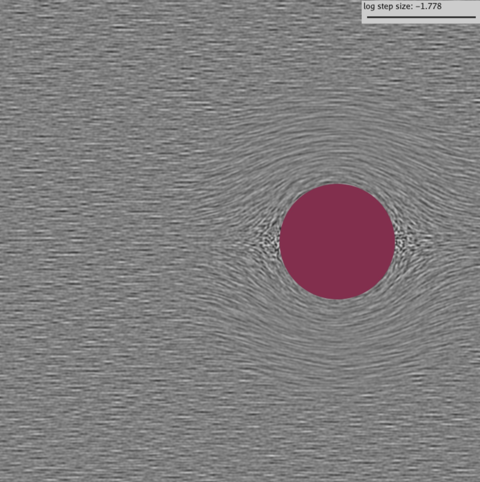
It’s nice to see the field you are designing rather than having to wait for the particles to advect through it. You can use the line integral convolution code from the lecture demo to draw the field in the background, which may be helpful in setting up the next part. If you copy that in and run it on the laminar flow field you should get something like this.
2.2 Single band curl noise
Now to the turbulence part! Import the 2D Perlin noise \(N(\mathbf{x})\) from the lecture demo, and set the potential to call this function. You will find the velocity is really slowly varying, and this is because the noise is at too large a length scale.
When using procedural noise we describe a noise as being at a particular scale or frequency; for the purposes of this assignment we will define “noise with scale \(s\)” to mean \(sN(\mathbf{x}/s)\). We scale the result of the noise by \(s\) so that its derivative will still have the same magnitude.
Here is curl noise at scale 0.1 visualized with LIC.
2.3 Multi-band turbulence
Turbulence in real fluids is a multi-scale phenomenon, with swirling eddies at a whole spectrum of scales. In particular, the famous Kolmogorov spectrum tells us to expect kinetic energy per unit mass at scale \(s\) to be proportional to \(s^{\frac{5}{3}}\), so the velocities should scale as the square root of energy, or \(s^{\frac{5}{6}}\).
In our simulation of turbulent fluids, the velocity of one band of turbulent flow / curl noise is a scalar amplitude \(v\) applied to the entire potential field \(v sN(\mathbf{x}/s)\), which then also makes the velocity proportional to \(v\).
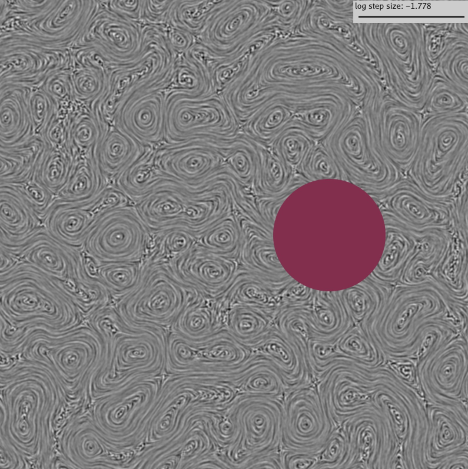
Eventually, we would like to add together a number of noise functions at different scales and velocities. We will have a number of bands indexed by \(i\); the scale of band \(i\) is \(s_i = 2^{-i}s_0\) and the velocity of band \(i\) is \(2^{-5i/6} v_0\). Here is an example of a multi-band curl noise that is computed using four bands starting at \(s_0 = 0.2\) and \(v_0 = 0.25\). (\(a_i\) in the Bridson paper is equivalent to \(v_i \cdot s_i\), while \(d_i\) in the paper corresponds to \(s_i\) here).
2.4 Putting it all together
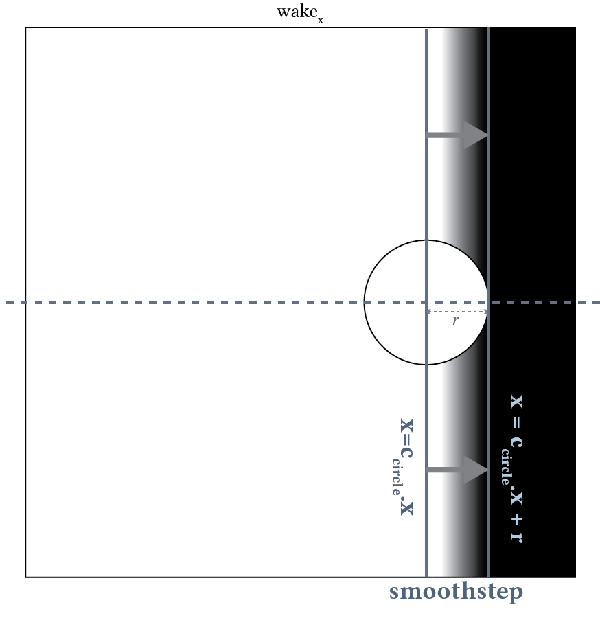
Now we have almost all the pieces to build our flow with a turbulent wake behind the obstacle. We only need a smooth window function that we can multiply the turbulence by so that it only affects the desired area behind the obstacle. For this Bridson used a product of three smoothstep functions that ramp down the turbulence at the top, bottom, and right sides of the wake.
You can compute this window in two steps:
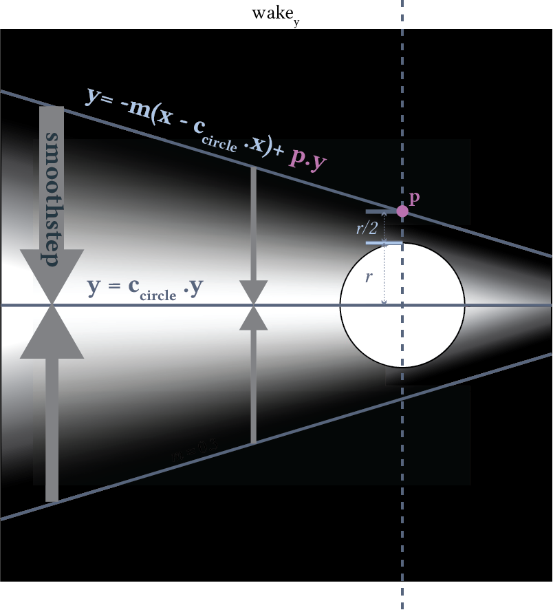
First, get the product of two smoothstep functions whose nonzero region is visualized with grayscale values in the \(\mathrm{wake}_y(\mathbf{x})\) figure
Second, get the smoothstep function along x direction as shown in the \(\mathrm{wake}_x(\mathbf{x})\) figure.
The product of \(\mathrm{wake}_x(\mathbf{x})\) and \(\mathrm{wake}_y(\mathbf{x})\) becomes the window \(A(\mathbf{x})\) we desire, and if visualized as grayscale, it looks like this.
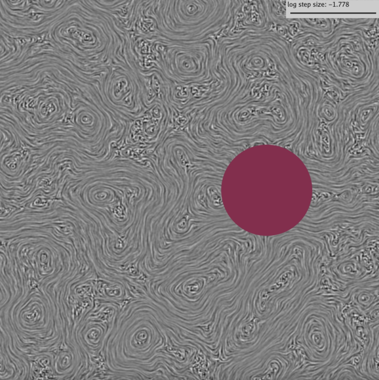
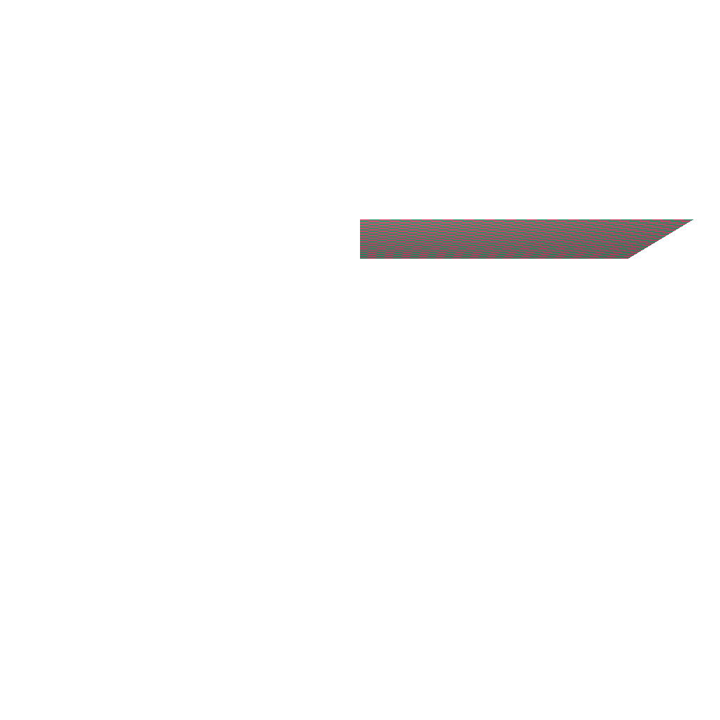
Finally assemble the four pieces (background, object influence, turbulence, and window) as described above to produce the complete field. If you advect particles through this field you should get something like this.
2.5 Time varying flow
This flow looks nice for a while but it is boring and unrealistic how it stays steady over time; real turbulence is always evolving. It is simple to fix this: promote the noise from 2D to 3D and pass the time as the third coordinate! It is good to scale the time in the same way as the \((x,y)\) coordinates so that the small eddies evolve faster than the large ones.
With just that one change you can get more interesting motion (computed using time scale \(0.03s\) for length scale \(s\)).
2.6 Optional extras
For a modest amount of extra credit, do something cool with this system that we didn’t specify! Some ideas:
- Make a flow around multiple obstacles of different shapes.
- Make a flow for steam billowing out of a smokestack.
- Make an animation of the smoke that rises from an incense stick or snuffed-out candle, which flows in a smooth column for a while and then becomes turbulent, slows, and spreads horizontally.
3 Second part: Mass-spring cloth simulation
For the second part, you will implement a simple cloth simulator
where a square piece of cloth collides with an object. The starter code
mass_spring_cloth.py provides mesh constrution and
rendering for the scene.
If you have not done so for the first part, you will need to run
pip install pywavefront to install the package needed for
reading the spherical collision object.
3.1 Cloth initialization
A piece of square mass-spring cloth is composed of \(N\times N\) (evenly-spaced) particles connected by varying types of springs. We use \([i,j]\ (0\leq i,j < N)\) to denote the particle located at \(i^{th}\) row and \(j^{th}\) column. Each particle has the following states:
Mass \(m\). Here we set \(m\) to be constant and assume that all particles have the same mass of \(\frac{1}{N\times N}\).
Position \(\mathbf{x}_{i,j}(t)\)
Velocity \(\mathbf{v}_{i,j}(t)=\dot{\mathbf{x}}_{i,j}(t)\)
The position and velocity are affected by different forces which we will implement in subsequent steps, and follow Newton’s second law: \[ \mathbf{a}_{i,j}(t)=\dot{\mathbf{v}}_{i,j}(t) = \ddot{\mathbf{x}}_{i,j}(t)=\frac{\mathbf{F}_{i,j}(t)}{m}\]
You will use Symplectic Euler to update the positions of the particles.
The first task is simple: Initialize the cloth by setting the
particle positions in the Taichi kernel init_cloth(). In
the starter code we have defined a Taichi field of \(N\times N\) 3D vectors called
x that holds the positions of the \(N^2\) particles. You will need to set the
values of this field, referring to the particles by their \([i,j]\) indices. The cloth should have
width and height of 1. The demo has the cloth quad initialized on the
\(y=0.6\) plane, but you can adjust its
position as desired.
The particle positions from x are read by
update_vertices(), where the particle positions are simply
copied to the mesh vertex positions.
The result should look like this where \(N=128\).
To make sure you are indeed getting a full quad, move the camera by dragging the left mouse button in the GUI.
3.2 Springs
There are three types of springs that connect the particles. For an arbitrary particle at \([i,j]\), there are (at most) 12 connections established as follows:
Structural: (At most) four neighboring particles at \([i,j+1],[i,j-1],[i+1,j],[i-1,j]\)
Shear: (At most) four neighboring particles along the diagonal at \([i+1,j+1],[i+1,j-1],[i-1,j+1],[i-1,j-1]\)
Flexion: (At most) four particles that are two particles away at \([i,j+2],[i,j-2],[i+2,j],[i-2,j]\)
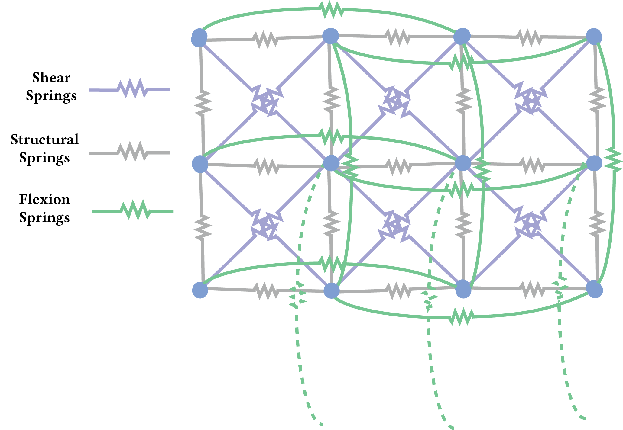
The illustration above demonstrates how the different kind of springs are attached to the particles of a 2D grid.
Each type of string has a different stiffness, denoted by \(k_0\) (structural), \(k_1\) (shear) and \(k_2\) (flexion). Make GUI sliders for each stiffness and play with the parameters to see how they affect the cloth.
We assume that the cloth is initially at rest, so you can calculate the rest lengths of a spring by the distance between the particles connected by the spring in the initial state.
3.3 Forces
3.3.1 Spring forces
For two particles at positions \(\mathbf{x}_1,\mathbf{x}_2\) connected by a spring of stiffness \(k_{\text{spring}}\) with rest length \(l_0\), the spring force acting on the particle at position \(\mathbf{x}_1\) is \[F_{\text{spring}}=k_{\text{spring}}(\|\mathbf{x}_{12}\| - l_0)\hat{\mathbf{x}}_{12}\] where \(\mathbf{x}_{12} = \mathbf{x}_2 - \mathbf{x}_1\) and \(\hat{\mathbf{x}}_{12}\) is the unit direction of \(\mathbf{x}_{12}\).
3.3.2 Gravity
The gravity acting on each particle is simply \(\mathbf{F}_{\text{gravity}}=\begin{bmatrix}0& -mg& 0\end{bmatrix}\) where \(g=9.81\).
Additionally, you will write the time stepping function following Newton’s second law. You will need to create a vector field for storing the velocities of particles, in addition to storing the positions in part 1. Pin the positions of the particles at indices \([0,0]\) and \([0,N-1]\), by simply setting their velocities to zero in the integration.
After implementing spring forces and gravity as well as setting up the time stepping function, your result should look like this. The demo has \(k=3*N\) for all the stiffnesses. Note that the result in this and subsequent videos are generated at 60 frames per second, while the simulation (and the FPS shown in the GUI) might be much slower, depending on your hardware.
3.3.3 Damping
Now we will add some damping so that the simulation converges. There are two types of damping:
- Spring damping: For two particles at positions \(\mathbf{x}_1,\mathbf{x}_2\) connected by a spring of stiffness \(k_{\text{spring}}\), the damping force corresponding to the spring force acting on particle at position \(\mathbf{x}_1\) is
\[\mathbf{F}_{\text{spring_damp}}=k_{\text{spring_damp}}(\mathbf{v}_{12}\cdot\hat{\mathbf{x}}_{12})\hat{\mathbf{x}}_{12}\] where \(\mathbf{v}_{12} = \mathbf{v}_2 - \mathbf{v}_1\)
- Viscous damping: \[\mathbf{F}_{\text{viscous_damp}}=-k_{\text{viscous_damp}} \mathbf{v}_{1}\]
Again, make GUI sliders for the two damping parameters \(k_{\text{spring_damp}}\) and \(k_{\text{viscous_damp}}\) and observe the effects of changing the parameters. Your result should look like this. Here, \(k_{\text{spring_damp}}=0.0384\) and \(k_{\text{viscous_damp}}=\frac{1}{N^2}\).
3.4 Collision with a sphere
Now we will bring in a sphere and have it collide with the cloth. During the integration, for each particle, check if the distance from the center of the sphere is smaller than the sphere radius. If the normal component of the velocity is into the surface, project the velocity to the tangent plane of the sphere at the contact point; if the normal component of the velocity is away from the surface let it be, i.e. \[\mathbf{v}\leftarrow \mathbf{v}-\min(0,\mathbf{v}\cdot\mathbf{n})*\mathbf{n}\] Here, \(\mathbf{n}\) is the surface normal vector at the particle position. The result looks like this.
3.5 Extra features (optional)
- Explore with different types of collision objects, e.g. shapes other than the sphere, or even arbitrary meshes.
- Explore the parameter space of the mass spring system, and set up the parameters to replicate the behavior of a certain material such as silk or cardboard.
4 Submission
You need to include two things in your submission:
- A pdf file including a link to the chosen commit for your submission. If you submit a direct link to your repository, we would assume that you would like us to look at your latest commit.
- A demo video demonstrating the functionalities of your simulators (please make sure that we can easily run your code and generate similar results shown in the demo).