| Background | History | Algorithms | Cascade Correlation |
| Home |
| Proteins |
| Neural Networks |
The Cascade Correlation Algorithm
Developed in 1990 by Fahlman, the cascade correlation algorithm provides a solution. Cascade correlation neural networks are similar to traditional networks in that the neuron is the most basic unit. Training the neurons, however, is rather novel. An untrained cascade correlation network is a blank slate; it has no hidden units. A cascade correlation network’s output weights are trained until either the solution is found, or progress stagnates. If a single layered network will suffice, training is complete.
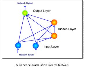 If further training yields no appreciable
reduction of error, a hidden neuron is ‘recruited.’ A pool of hidden neurons
(generally 8) is created and trained until their error reduction halts. The
hidden neuron with the greatest correspondence to the overall error (the one
that will affect it the most) is then installed in the network and the others
are discarded. The new hidden neuron ‘rattles’ the network and significant
error reduction is accomplished after each hidden neuron is added. This
ingenious design prevents the moving target problem by training feature
detectors one by one and only accepting the best. The weights of hidden neurons
are static; once they are initially trained, they are not touched again. The
features they identify are permanently cast into the memory of the network.
Preserving the orientation of hidden neurons allows cascade correlation to
accumulate experience after its initial training session. Few neural network
architectures allow this. If a back-propagation network is retrained, it
‘forgets’ its initial training.
If further training yields no appreciable
reduction of error, a hidden neuron is ‘recruited.’ A pool of hidden neurons
(generally 8) is created and trained until their error reduction halts. The
hidden neuron with the greatest correspondence to the overall error (the one
that will affect it the most) is then installed in the network and the others
are discarded. The new hidden neuron ‘rattles’ the network and significant
error reduction is accomplished after each hidden neuron is added. This
ingenious design prevents the moving target problem by training feature
detectors one by one and only accepting the best. The weights of hidden neurons
are static; once they are initially trained, they are not touched again. The
features they identify are permanently cast into the memory of the network.
Preserving the orientation of hidden neurons allows cascade correlation to
accumulate experience after its initial training session. Few neural network
architectures allow this. If a back-propagation network is retrained, it
‘forgets’ its initial training.
The size step problem contributes greatly to error stagnation. When a network takes steps that are too small, the error value reaches an asymptote. Cascade correlation avoids this by using the quick-prop algorithm. Quick-prop finds the second derivative (change of slope) of the error function. With each epoch it takes a different size step corresponding to the change of the error slope. If the error is reducing rapidly, quick-prop descends quickly. Once the slope flattens out, quick-prop slows down so that it does not pass the minimum. Quick-prop is like a person searching for a house. If the person knows he is far away, he drives fast. Once he approaches the house, he slows down and looks more carefully
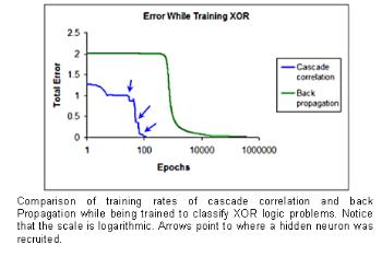
The difference in training speeds is unmistakably clear from an analysis of back-propagation’s error graph versus that of cascade-correlation. Back-propagation slowly converges on a solution as the moving target problem and size-step problem strike. In some trials the hidden neurons become locked on the same feature, and the network never attains a solution. As visible in the graph, cascade correlation faces this same problem except that when the error reduction stagnates, cascade correlation recruits a new hidden neuron that will promote further error reduction. Cascade correlation aggressively seeks to reduce error at the fastest possible rate.
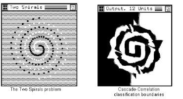 The cascade correlation algorithm trains substantially
faster then virtually any other existing algorithm. A classic
classification benchmark, the two spirals problem developed by Alexis Wieland,
clearly illustrates this. The two spirals problem consists of 194
points arranged in a circular pattern; half the points are of type A, the other
half are type B. A heavily modified version of back-propagation took 20,000
epochs and 1.2 billion weight modifications to converge on a solution. Cascade
correlation takes an average of 1700 epochs and a mere 19 million alterations.
The cascade correlation algorithm trains substantially
faster then virtually any other existing algorithm. A classic
classification benchmark, the two spirals problem developed by Alexis Wieland,
clearly illustrates this. The two spirals problem consists of 194
points arranged in a circular pattern; half the points are of type A, the other
half are type B. A heavily modified version of back-propagation took 20,000
epochs and 1.2 billion weight modifications to converge on a solution. Cascade
correlation takes an average of 1700 epochs and a mere 19 million alterations.