 |
Geometric Objects in QMG
|
The QMG package supports two datatypes:
breps and
simplicial
complexes. Simplicial
complexes are also called “meshes.”
Before plunging into the details of geometric representation,
consider using some of the simpler ways to create breps.
For a simple way to create two-dimensional breps, consider the
gm_cpoly
routine. For a simple way to create three-dimensional polyhedral
breps,
consider using OFF format.
A brep is a geometric object that is specified by its
boundary faces (“brep” is short for
“boundary representation”). Many
people pronounce brep like “bee-rep”.
Breps have different internal
representations in Matlab versus Tcl/Tk, but the two representation
have essentially the same data.
Below we describe the
details of the internal representations, but first we describe
data present in a brep.
The next few paragraphs cover three-dimensional
breps whose intrinsic dimension is also three. Below
we turn to lower-dimensional breps.
A brep is composed of topological entities which are
also sometimes called faces for short. A brep has
four types of faces: chambers, surfaces,
edges and vertices. These faces have dimensions
3, 2, 1, 0 respectively.
The boundary of each face is defined
by a list of faces of one lower dimension. In other words, the
boundary of a chamber is one or more surfaces, the boundary of
a surface is zero or more edges, and the boundary of an edge
is zero or more vertices.
The topological hierarchy for a QMG 2.0 object must have the following
property: if two faces have a common point, then their intersection
must be a common topological subentity. For example, a cube is bounded
by six squares. Two adjacent squares must have a common topological
edge.
Breps in QMG 2.0 must be finite and must be watertight. Watertight
has the following meaning in 3D:
for each chamber C, when
all the edges that occur as boundaries of surfaces that occur
as boundaries of C are enumerated,
each edge must occur an even number
of times (counting multiplicity).
Similarly, for each surface S, when all the vertices that occur
as boundaries of edges that occur as boundaries of S
are enumerated,
each vertex must occur an even number of times in this enumeration.
For example, this rule means that for the cube mentioned
in the last paragraph, it is not permissible for two surfaces that share
a common edge to own separate copies of that edge under two different
names.
Each topological entity, except for a chamber,
is composed of geometric entities. In particular, a surface is composed
of Bezier patches, an edge is composed of Bezier curves,
and a vertex has a point associated with it.
Bezier patches of two types are supported: triangular patches
and tensor product patches. See G. Farin, Curves and Surfaces
for Geometric Design for the definition of the two kinds of
Bezier patches. Here are
the rules governing Bezier patches and curves.
-
The parametric domain for a triangular patch is the
{(u,v):u+v≤1;
u≥0; v≥0}. The parametric
domain for a quadrilateral patch is {(u,
v): 0≤u,v≤1}.
The parametric domain for a curve is [0,1].
-
The control points for a curve are numbered so that
p(0) is the first-listed (indexed 0)
control point and p(1) is the
last-listed (indexed d), where p is the degree-d
parametric function.
-
The control points for a triangular
patch are ordered according to the following
example for a degree-3 patch:
|
u=0,v=1
|
|
|
|
|
|
|
|
0
|
|
|
|
|
|
1
|
2
|
|
|
|
|
3
|
4
|
5
|
|
|
|
6
|
7
|
8
|
9
|
|
u=0,v=0
|
|
|
|
|
u=1,v=0
|
-
Control points for a quadrilateral patch are numbered according to
the following degree-(3,2) example:
|
u=0,v=1
|
|
|
|
|
u=1,v=1
|
|
|
8
|
9
|
10
|
11
|
|
|
|
4
|
5
|
6
|
7
|
|
|
|
0
|
1
|
2
|
3
|
|
|
u=0,v=0
|
|
|
|
|
u=1,v=0
|
-
Patches and curves must be nondegenerate, meaning that the
parametric function must be injective on its domain, and that
the derivative must be full-rank at every point of the
domain. (Note that certain domains, such as cones, have
points on curved surfaces where the derivative
becomes low-rank. Such domains cannot be represented
with order higher than first in QMG 2.0.)
-
If two distinct patches have a common point, then the common point must
either be a vertex, or else the two patches must have a common
bounding curve.
-
Two patches are assumed to be adjacent along an edge if the two
extreme control points of the common edge are in common. Thus,
adjacency between patches is determined with a purely combinatorial test.
Patches of different degrees can be adjacent.
(See
test9 for an example of a degree-1 patch against
a degree-3 patch.)
Nonetheless,
there cannot be any gap between the patches, meaning that the
parametric function of the
higher-degree neighbor must degenerate to a
lower degree along the common edge.
This requirement also means that two distinct
Bezier curves cannot have both endpoints in common with each
other.
-
The dihedral angle between two adjacent patches may not be zero
at any point along their common edge.
Rules concerning the relationship between topological entities
and geometric entities are as follows:
-
The topological boundary of a face F must be made up of
entities that are exactly the boundary of
the geometric entities making up F.
For example, a surface
is shaped like a square with a small hole or slit in the
middle cannot have a single quadrilateral
patch as its only geometric entity.
-
Faces must be orientable, i.e., there must be a globally consistent way
to orient the patches of a face. In particular, a face shaped
like a Moebius strip is not allowed.
-
Faces are supposed to be G1 (meaning that the
normal varies continuously on the topological entity, even as patch or
curve boundaries are traversed).
But small deviations
from G1 are permitted.
For example,
a topological surface composed of noncoplanar linear
triangles is allowed, as long as the dihedral angles
between neighboring triangles are near 180 degrees.
See the
curvecontrol option
to the mesh generator.
-
In QMG 2.0, toplogical faces must be connected.
In QMG, each face is allowed to have property-value pairs. This is
a list of pairs of strings. The first string in each pair is the property
name, and the second string is the value of that property.
For example, surfaces can
have a color property that indicates their color
to be used by graphics routines.
Property names are case-insensitive, e.g., color and
CoLOR are not distinguished.
The brep itself can have
property-value pairs that apply to the whole brep. One important
global property is geo_global_id. The corresponding value
for this property is intended to be a universally unique ID string
for the brep. In QMG 2.0, there is no system for generating these
ID strings, but some of the routines
like gmchecktri
check them.
So far we have discussed breps with intrinsic and embedded dimension
equal to 3. The embedded dimension of a brep is the
dimension in which it is embedded and is equal to the number of
coordinates in each of its control points. QMG 2.0 supports either
2 or 3 for this value. A brep's intrinsic dimension is the highest-dimensional
face that it owns. For instance, a brep with topological vertices and
edges but no surfaces or chambers would have intrinsic dimension equal
to 1. The intrinsic dimension can never exceed the embedded dimension.
The mesh generator requires that the intrinsic and embedded dimensions
be equal, although other routines in QMG 2.0 allow the intrinsic
dimension to be lower.
If the intrinsic and
embedded dimension of the brep are both d
(where either d=2 or d=3)
then the term region is used to denote the topological
entities
of dimension d.
Thus, for a three-dimensional brep, its chambers
are its regions. For a two-dimensional brep, its surfaces (subsets
of the plane) are its regions. Regions are completely specified
by their boundaries, so they do not have any
geometric
entities
associated with them in a brep definition.
Thus, the data items that make up a brep are as follows.
-
Two integers: its embedded and intrinsic dimension.
-
Its global property-value pairs.
-
A table of control points.
-
Its faces (topological entities). Faces are listed in increasing
order of dimension (i.e., vertices first, etc).
Each topological entity has five data items associated with
it:
-
The face name, which is a string.
-
Property-value pairs of the face (a list of ordered pairs of strings).
-
The boundary of the face, which is a list of faces of one lower
dimension. This list may be empty if the face is closed
(such as
a sphere). Each bounding face in this list is
accompanied by the specification of its orientation with respect
to the parent face: inward, outward, or no orientation specified.
This orientation information is currently not used by QMG.
-
The list of faces of two or more dimensions lower that are
internal boundaries. See below.
-
The geometric entities making up the face.
Regions cannot have geometric entities; on the other hand,
every other face must have at least one geometric entity.
A geometric entity
is specified by
-
its type (vertex, curve, triangle, or quadrilateral),
-
its degree (for a curve or triangle) or degree-pair (for
a quad), and
-
its list of control points (integer indices into the control point
table) in the correct order described above.
The preceding section detailed geometric and topological entities, but the
reader may wonder why we bothered with this distinction. Why not have
geometric entities only? There are two advantages to this system:
-
Property-value pairs are associated with topological entities. This
means that many geometric entities can be grouped together with a single
finite element boundary condition (for example).
-
The mesh generator respects boundaries between topological entities
but not between geometric entities. This has important consequences
in practice, and you should design your domains with this
fact in mind.
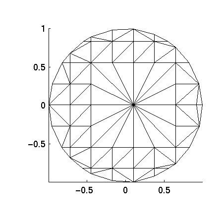
For example, consider the following regular 30-gon.
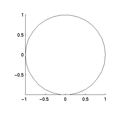 Two possible ways to represent this in QMG would be:
-
as a domain with a
single topological edge as its boundary. That edge
is made up of
30 linear Bezier curves, or
-
as a domain with 30 topological edges on the boundary. Each topological
edge made up of one linear Bezier curve.
In the first case, the topological edge is not
G1, but nonetheless QMG permits small
divergences from G1 as mentioned earlier.
There are also many other options for representing
the 30-gon; for example, there could be
five edges each made of six linear curves, etc.
Here is the mesh generated by QMG (coarse mesh requested) for the first
option:
Here is the mesh generated by QMG (coarse mesh requested) for the
second option:
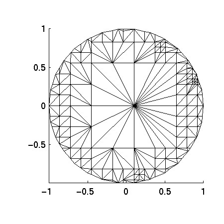 Notice the two meshes are quite different. Depending on your application,
one or the other might be more appropriate.
As mentioned early, a brep face can have bounding faces of one lower
dimension.
A brep face can also have internal boundaries,
which are subfaces of lower dimension that are inside the face
itself, i.e., they have the interior of the face on both sides
of them.
Notice the two meshes are quite different. Depending on your application,
one or the other might be more appropriate.
As mentioned early, a brep face can have bounding faces of one lower
dimension.
A brep face can also have internal boundaries,
which are subfaces of lower dimension that are inside the face
itself, i.e., they have the interior of the face on both sides
of them.
Internal boundaries usually serve one of two purposes in a scientific
computation: they act as demarcations between separate regions
of the domain (for instance, the domain may represent an object
that is a composite of several materials) or they act as
singular boundaries, for example, in modeling a region
with a slit or crack.
Holes in a domain are not internal boundaries—they
are classified as ordinary boundaries.
Internal boundaries are useful because the mesh generator will
respect them in its mesh (i.e. mesh elements will not cross through
them). They can also be the site of boundary conditions for the
finite element package.
There are three kinds of internal boundaries supported by the QMG
package, multi-region, repeated boundary, and low-dimensional
boundary.
A multi-region brep means that there are multiple regions
in the brep. (Recall that region means a topological entity
of dimension equal to the embedded dimension.)
The boundary between two regions is a type of internal boundary. The
region on either side sees it as an ordinary boundary.
A repeated boundary means that a region has a boundary
face listed twice in its list of boundaries. For example,
suppose a 3D chamber lists a topological surface twice in
its list of bounding faces. This makes the surface act like
a crack or fissure inside the chamber. Lower-dimensional
faces can also have repeated boundaries. This is sometimes
necessary to attach a region's repeated boundary to an exterior boundary.
For instance,
to represent a cube with a crack, such that the crack meets
an exterior boundary, the crack itself would be a repeated
boundary of the region, and then its edge where it meets the
exterior boundary would be a repeated boundary of the exterior
boundary.
Finally, a face can have one or more low-dimensional boundaries,
which act like low dimensional cracks. In particular, a chamber
can have edges or vertices as low-dimensional boundaries, and
a surface can have vertices as a low-dimensional boundaries.
Multi-region breps are generally used for the case of internal
boundaries that demarcate the brep into several zones.
The mesh generator lists the elements that it generates
according to the region in which they lie.
See the description of meshes below.
The finite element program can take advantage of these labels during
matrix assembly. For example, it can use different functions to
compute conductivity and source terms for the two sides
of the internal boundary corresponding to different materials.
In the case of a single-region brep with repeated boundaries,
there is no concept of one side of
the internal boundary versus the other since the fissure may cut
only partway through the domain. Thus, all elements have the
same label.
The various types of internal boundaries can be freely
mixed in the same brep.
The mesh generator will produce a single layer of nodes
along either an repeated boundary or an
internal boundary in a multi-region domain. In some applications
a double layer of nodes is desirable. It is possible
to produce a double layer of nodes along a repeated boundary
with the
gmdouble
function.
A simplicial complex is a collection of simplices of one specific
dimension embedded in a space of the same or higher dimension. (Thus,
simplicial complexes in QMG cannot contain
simplices of several different dimensions in the same complex).
Simplicial complexes are the output of the mesh generator and are an
input to the finite-element program and to the graphics programs.
As with a brep, a simplicial complex has two integers associated
with it, the embedded dimension and the intrinsic dimension.
Also like a brep, a simplicial complex can have property-value pairs.
For example, one possible property name is geo_global_id.
The mesh generator stores the brep's ID in this field during
mesh generation. The field is omitted in
a mesh generated for a brep without a global ID.
The rest of the data is lists of
vertices and elements.
The first list is the vertex real-space coordinates. Each vertex has
a global ID number, which must be a nonnegative integer. Global ID
numbers must be unique within the mesh but
do not have consecutive or in order. With each global ID is
a tuple of two or three real-space coordinates of the node. (The number
of real-space coordinates per node equals the embedded dimension.)
Next are lists of vertices and simplicial faces associated with brep
topological
entities. Let d be the embedded dimension of the mesh.
Let B be the brep that gave rise to the mesh.
Then each brep topological entity F of dimension 0 to
d−1 has a list of vertices lying on it.
For each vertex on F, the following information is
stored: its global ID number, the curve or patch index of
the geometric entity containing the vertex (omitted when d=0)
and the parametric coordinates on that entity (omitted when d=0).
Mesh vertices lying on lower-dimensional subfaces of
F are also listed as lying on F since they
will have a different patch-index and parametric coordinates
with respect to F. Thus, the same mesh vertex may appear in
many different lists associated with various brep faces.
Each brep topological entity of dimension 1 to d has
a list of simplex faces lying on it. This list is made of tuples.
A brep entity of dimension k contains
tuples made up of k+1 vertices. These vertices are listed
via their global ID numbers. For faces of dimension 1 to
d−1, all vertices listed in any of these
tuples must also be listed as a vertex of the face as in
the previous paragraph.
The full-dimensional simplex faces (i.e.,
the case k=d) are the actual simplices of the
mesh.
Two geometric properties of meshes
An important property of a simplex
is its aspect ratio. The aspect
ratio of a simplex can be defined in several ways, which are
all equivalent up to constant multiples. In the QMG package,
aspect ratio of a simplex is defined as the ratio of the length of its
longest edge divided by its shortest altitude.
Small aspect ratios are desirable because large aspect ratios
cause a loss of accuracy in the finite element approximation,
and can also lead to condition number problems for the
assembled stiffness matrix.
All full-dimensional simplices should to have the correct
orientation. Let v0, ...,
vd
be the vertices of a simplex.
The correct orientation is defined as follows. Form
the d×d
matrix whose ith row is vi−v0
(a d-vector). The determinant
of this matrix must be positive. In two dimensions, this means
that the vertices are listed in counterclockwise order. In three
dimensions this means that if you curl your right-hand around
v0, v1,v2,
then your thumb is pointing toward v3.
Both Matlab and Tcl/Tk versions of QMG support Ascii format. In
particular, the gm_read
and gm_write
functions use this format. Furthermore, in Tcl/Tk, conversion
to Ascii format is automatic for any operation that causes
string format to be released. (See below
for more information.)
Ascii format consists of free-form plain text with parentheses
as delimiters. Free-form means that linebreaks are usually not significant,
except that they act like spaces. Comments are marked with a '#'
sign. A comment may start at any position in the line, and is
in effect until the end of the current line.
The Ascii format for a brep follows the following grammar. In this grammar,
normal-weight text denotes field names and boldface denotes literals.
The symbol
:= indicates substitution for a field name.
The vertical bar symbol | means
either/or, and curly braces {} indicate optional data. Parentheses when
indicated are literals (i.e., parentheses occur in the corresponding place
in the actual brep).
-
asciiBrep := code intrinsicDim embeddedDim globalPropVal controlPoints
vertexList {edgeList {surfaceList {chamberList}}}
-
code := brep_v2.0
-
intrinsicDim := 0 | 1 |
2 | 3
[Intrinsic dim must be less than or equal to embedded dim.]
-
embeddedDim := 2 | 3
-
globalPropVal := ( prop1 val1 ...
propm valm )
[The property/value pairs are arbitrary strings. If
property or value strings contain
space, then there must
be an outer pair of parentheses to delimit the string.
Currently, the only global property value with significance to
QMG 2.0 is geo_global_id.]
-
controlPoints := ( entry1 ... entrym )
[The number of entries m must be a multiple of the
embedded dimension e.
Each entry in this list is a floating-point number
possibly in scientific notation. There are a total of
m/e control points, with each control point's coordinates being denoted
by e consecutive entries in this list.]
-
vertexList := faceList; edgeList := faceList; surfaceList := faceList;
chamberList := faceList. [The number of such lists must equal
the intrinsic dimension plus 1. For example, if the intrinsic dimension
is 1, then the brep must have a vertexList and an edgeList but
cannot have a surfaceList nor a chamberList.]
-
faceList := (name1 propVal1
boundary1 lowdim1 geom1 ...
namen
propValn
boundaryn lowdimn
geomn)
[In other words, each brep face has five entries in its
face list: name, propVal, child, lowdim, geom.
The name field is an arbitary string. A name field with spaces
should be enclosed in parentheses. The remaining
fields are as follows.]
- propVal := (prop1 name1 ...
propm namem)
[As above, these can be arbitrary string, although
parentheses should be used for strings with spaces.]
- boundary := (childname1 ...
childnamem)
[These are names of bounding faces. That is, these names refer
to the names appear in the 'name' field of the lower-dimensional
faces. Names appearing in this list must be faces of exactly one
lower dimension. Each childname can optionally be preceded
by the symbol + or - to indicate orientation. Orientations
are not used by QMG 2.0.]
- lowdim := (childname1 ...
childnamem)
[These are the names of the low-dimensional bounding faces.
Names appearing in this list must be faces of dimension lower by
2 or 3 from the dimension of the face.]
- geom := (geoentity1 ...
geoentitym)
- geoentity := (vertex cpnum) |
(bezier_curve deg cpnum1 ...
cpnump) |
(bezier_triangle deg cpnum1 ...
cpnump) |
(bezier_quad deg1 deg2
cpnum1 ... cpnump).
[The vertex entity is allowed only for topological
vertices, and a topological vertex must have exactly one such
entity. The bezier_curve
entity is allowed only for edges. The
bezier_triangle and
bezier_quad entities are allowed only for surfaces.
The degree entries are positive integers. The number of
control points p is deg+1 for a curve, (deg+1)*(deg+2)/2
for a triangle, and (deg1+1)*(deg2+1)
for a quad. Each
control point
cpnum1, ..., cpnump is a nonnegative integer
that is an index into the control point list.]
The Ascii format for a mesh is:
-
asciiMesh := code intrinsicDim embeddedDim globalPropVal vertexList
brepVertexList
brepEdgeList {brepSurfaceList {brepChamberList}} [The number
of brep entity lists must be the intrinsic dimension plus 1.
In other words, if the mesh's intrinsic dimension is 1, then
it must possess a brepVertexList and a brepEdgeList but may
not possess a brepSurfaceList nor a brepChamberList.]
-
code := mesh_v2.01
-
intrinsicDim := 1 |
2 | 3
[Intrinsic dim must be less than or equal to embedded dim.]
-
embeddedDim := 2 | 3
-
globalPropVal := ( prop1 val1 ...
propm valm )
[The property/value pairs are arbitrary strings. If
a property or value string contains spaces, then it
should be enclosed in an outer pair of parentheses.
Currently, the only global property value with significance to
QMG 2.0 is geo_global_id.]
-
vertexList := (
globalId1 xc1 yc1
{zc1} ...
globalIdn
xcn ycn
{zcn})
[This is a list of the n nodes in the mesh. Each
entry consists of a global ID, which must be a nonnegative
integer, followed by either 2 or 3 coordinates, which are
real numbers. The number of coordinates is equal to the
embedded dimension (2 or 3). The global ID's do not have
to be in increasing order, but they must be distinct.]
-
brepVertexList := ((globalId1) ( ) (globalId2) ( ) ...
(globalIdm) ( )) [This is the list of mesh entities
associated with the brep's vertices. There is one globalId per
brep vertex.]
-
brepEdgeList := (edgeVlist1 edgeSlist1 ...
edgeVlistm edgeSlistm)
[This is the list of mesh entities associated with the
brep's edges. In particular, there is an edgeVlist and edgeSlist
for each brep edge, so m here denotes the number of
brep edges.]
- edgeVlist :=
(globalId1 curveindex1 paramcoord1 ...
globalIdp curveindexp
paramcoordp)
[This is the list of mesh nodes lying on a particular brep edge.
Each triple in this list specifies which mesh node, which geometric
curve within the brep edge, and the parametric coordinate
(a real number in [0,1]) of the mesh node.]
- edgeSlist :=
(globalId1 ... globalId2r)
[This is a list of global node ID's. They are arranged in
pairs, for a total of r pairs. Each pair indicates
the endpoints of a mesh edge that lies on the brep edge.
The union of these mesh edges should equal the brep edge.
Each global vertex ID lying in this list must also occur
in edgeVlist.]
-
brepSurfaceList := (surfaceVlist1 surfaceSlist1 ...
surfaceVlistm surfaceSlistm)
[This is the list of mesh entities associated with the
brep's surfaces. In particular, there is a surfaceVlist and surfaceSlist
for each brep surface, so m here denotes the number of
brep surfaces.]
-
surfaceVlist := ( ) |
(globalId1 patchindex1 paramcoordU1
paramcoordV1 ...
globalIdp patchindexp
paramcoordUp
paramcoordVp)
[This is the list of mesh nodes lying on a particular brep surface.
If the embedded dimension is 2, then this list is required to be
empty, that is, ( ). If the embedded dimension is 3, then
this list is divided into four-tuples.
Each four-tuple includes the global ID of the vertex, the index
of the geometric patch containing the mesh node, and the parametric
coordinates within the patch of the mesh node.]
- surfaceSlist :=
(globalId1 ... globalId3r)
[This is a list of global node ID's. They are arranged in
triples, for a total of r triples. Each triple indicates
the endpoints of a mesh triangle that lies on the brep surface.
The union of these mesh triangles should equal the brep surface.
Each global vertex ID lying in this list must also occur
in surfaceVlist.]
-
brepChamberList :=( ( ) chamberSlist1 ... ( )
chamberSlistm)
[This is the list of mesh entities associated with the
brep's chambers (assuming the intrinsic and embedded dimension are both 3).
In particular, there is a chamberSlist
for each chamber, so m here denotes the number of
brep chambers.]
-
chamberSlist := (globalId1 .....
globalId4r)
[This is a list of global node ID's. They are arranged in
four-tuples, for a total of r four-tuples. Each four-tuple indicates
the endpoints of a mesh tetrahedron that lies in the brep chamber.
The union of these mesh tetrahedra should equal the brep chamber.]
The Matlab internal representation of objects uses zero-based array
addressing. This implemented via a Matlab class called "zba".
In a zero-based array, rows and column numbering starts with 0
instead of 1. Many array operations with which you are familiar
have been reimplemented for zba's. You can extend the operations
available for zba's by adding new routines
to the @zba subdirectory.
To convert an array to a zba, use the zba function. To convert
back, use the double function.
>> z = zba([3,5,7]);
>> z(0)

ans =

     3

>> y = double(z);
>> y(1)

ans =

     3
The user can directly access entries of these objects to
examine and modify a brep or mesh. Breps or meshes can also be
created directly by the user or with m-files. (This is in contrast
to QMG 1.0 and 1.1, in which the object was stored in 'chunk' format
and was accessible and modifiable only by using certain
accessor functions.)
The zba's in QMG are usually nested, with the outer level being
a cell array. Every level of indexing in a nested zba is zero-based.
A brep is represented by a zero-based cell column vector with 6+i
entries,
where i is the intrinsic dimension of the brep. (This
documentation assumes that you are already familiar with
subscripting of vectors, matrices, and cell arrays in Matlab.)
Say the brep is b. The entries of b are as follows.
-
b{0} is a string which is always 'brep_v2.0'.
-
b{1}
is the intrinsic dimension.
-
b{2} is the embedded dimension.
-
b{3} is the property-value list. This is a 2-by-k cell
array, where each cell entry is a string. In other words,
b{3}{0,0} is the first property, b{3}{1,0} is its value, and so on.
-
Entry b{4} is the control-point table. This is an e-by-m
matrix (with
zero-based numbering), where m
is the number of control points and e
is the embedded dimension of the brep.
-
Entry b{5} holds vertices, b{6} holds edges, b{7} holds surfaces,
and b{8} holds chambers. Not all of these entries are present; the
number present depends on the intrinsic dimension of the brep.
The format of these entries is as follows.
Each of b{d+5}, for d=0,...,3, is a 5-by-t cell
array,
where t denotes the number of faces of the particular dimension.
The cells are as follows.
-
b{d+5}{0,i} (for i between 0 and t-1) is the name of the
ith face (a string).
-
b{d+5}{1,i} is the property-value pair list of this face.
It is a 2-by-k cell array of strings, where k is the number
of property values.
-
b{d+5}{2,i} is the list of subfaces of the ith face. This is a
1-by-r cell array,
where r is the number of subfaces.
Each entry is a string with the name of the subface. This name
may optionally be preceded by + or - to indicate orientation
(current not used).
-
b{d+5}{3,i}
is the list of lower-dimensional
internal boundaries. This is a 1-by-s cell array,
where s is the number
of lower dimensional internal boundaries. Each entry is a string
with the name of the subface.
-
bd{d+5}{4,i}
is the cell array geometric entities making up the
face. This cell array is 3-by-p, where p is the number
of entities. Entry {0,j} of this cell array is
a string, either 'vertex', 'bezier_curve', 'bezier_triangle',
or 'bezier_quad'. As mentioned above,
the choice of entity type is restricted according to the face dimension.
Entry {1,j} of the cell array is the degree, either empty (for a vertex),
one integer (for a curve or triangle) or two integers (for a patch).
Entry {2,j} of the cell array is a vector of control point indices.
The length of this vector follows the rule mentioned
above.
The matlab format for a mesh is as follows. A mesh m is a zba
cell-vector with 6+i entries, where i
is the embedded dimension. The entries as follows.
-
m{0} is the string 'mesh_v2.01'.
-
m{1} is the mesh's intrinsic dimension.
-
m{2} is the mesh's embedded dimension.
-
m{3} is a 2-by-k cell array of strings, which hold
the property-value pairs of the mesh.
-
m{4} is the mesh's node list. This is a k-by-r matrix,
where
k=3 if the embedded dim is 2, else k=4
if the embedded dim is 3.
The number of columns r is equal to the number of vertices in
the complex. The first entry of each column is the vertex's global
ID, which must be a nonnegative integer (stored as a double though).
The remaining entries in each column are the vertex's real-space
coordinates.
-
Entry m{5} holds mesh entities
associated with brep vertices, m{6}
holds mesh entities associated with brep edges,
m{7} holds mesh entities associated with brep surfaces, and
and m{8} holds
mesh entities associated with brep chambers.
Not all of these entries are present; the
number present depends on the intrinsic dimension of the brep.
The format of these entries is as follows.
Each of m{d+5}, for d=0,...,3, is a 2-by-t cell
array,
where t denotes the number of brep
faces of the particular dimension.
The cells are as follows.
-
m{d+5}{0,i} is the list of vertices associated with the
ith topological entity of dimension d. This list of vertices
is a k-by-r matrix defined as follows.
If d=0, then k=r=1, and the single entry
is the global id of the mesh vertex lying on topological vertex.
If d=1, then k=3, and each column of this array corresponds
to a mesh node lying on the topological edge. The first entry in the
column is the mesh's global ID (a nonnegative integer
stored as a double), the second entry is the curve index of the
curve of the edge that contains the vertex (a nonnegative
integer stored as a double), and the third entry is the parametric
coordinate (a double in [0,1]) of the point within the curve.
If d=2, then k=r=0 when the embedded dimension is 2.
If d=2 and the embedded dimension is 3, then k=4. Each column
of m{d+5}{0,i} is a vertex lying on the ith topological surface.
The first entry is the vertex global ID, the next entry is
the index of the patch within the topological surface, and the
last two entries are the parametric coordinates of the mesh node
within that patch.
If d=3, then k=r=0.
-
m{d+5}{1,i} is a matrix of mesh nodes (nonnegative global ID's, which
are integers but are stored as doubles) making up the mesh entities
lying on the face. If d=0, this matrix is empty.
If d=1, then m{d+5}{1,i} is a 2-by-r
matrix of mesh nodes; each column in this matrix is a mesh edge
lying on the brep edge. If d=2, then m{d+5}{1,i} is a 3-by-r
matrix; each column is a mesh triangle lying on the brep surface.
If d=3, then m{d+5}{1,i} is a 4-by-r matrix; each
column is a tetrahedron.
Two file-formats for meshes and breps can be used in
Matlab/QMG. The
first is Ascii format: to read a brep or mesh from
a file in Ascii format, use gm_read. To write it
out to a file, use gm_write.
Breps and meshes can also be saved in Matlab's native mat-file
format using the save and load
commands.
In Tcl/Tk, breps and meshes are represented internally using
C data structures. This data structure is not documented
here; refer to the source-code files GeoFmt.h
and MshFmt2.h in the QMGROOT/src/tcl directory and the comments
in those files.
Breps and meshes are Tcl dual-ported objects, which means that
they stay in the C data structures until a command is executed
on the object that is unable to directly handle breps or meshes,
for instance, the concat function. Then the object is
converted to its string representation, which is the
Ascii format described above.
Converting a large object to Ascii can be very
expensive, so you should avoid Tcl operations that cause
a conversion unless you need them.
To make it easier to manipulate geometric objects in Tcl,
there are also the two functions gm_obj2list
and its inverse gm_list2obj. The former
is roughly equivalent to converting the object to Ascii format
and then replacing all parentheses that occur at outer levels
with curly braces so that entries can be indexed and modified using the
lindex and lreplace
functions of Tcl. (The gm_obj2list function does not
actually convert to a string on an intermediate step. Instead,
it converts directly to Tcl's internal list representation, which
is more efficient.)
The gm_list2obj operation inverts this procedure.
Two file-formats for meshes and breps are available in
Tcl/QMG. The
first is Ascii format. To read a brep or mesh from
a file in Ascii format, use gm_read. To write it
out to a file, use gm_write.
Breps and meshes can also be saved in a binary file format
based on the XDR standards. The functions for this purpose are
gmxdr_read and gmxdr_write.
This XDR format is platform independent because the XDR routines
handle byte-order issues.
This documentation is written by
Stephen A.
Vavasis and is
copyright ©1999 by Cornell
University.
Permission to reproduce this documentation is granted provided this
notice remains attached. There is no warranty of any kind on
this software or its documentation. See the accompanying file
'copyright'
for a full statement of the copyright.
Stephen A. Vavasis, Computer Science Department, Cornell University,
Ithaca, NY 14853, vavasis@cs.cornell.edu