Overview and Examples of QMG

From the point of view of software development, the three most difficult aspects of finite-element analysis are the geometric modeling tools, the mesh generator, and the finite-element system solver. The QMG package is intended to address mesh generation in two and three dimensions. It also has a few tools to assist in geometric modeling and an elementary finite-element solver that solves the sparse matrix equation with Matlab's backslash operator.

The QMG package consists of approximately 40 separate functions. The user of QMG invokes the functions through a console interface. QMG does not have its own console interface; instead it relies on the scripting capabilities of other software packages. Currently QMG runs inside two different scripting environments: Matlab and Tcl/Tk. In addition, the user can invoke QMG directly from the shell in either Windows or Unix.

Also provided are a suite of examples demonstrating the use of many of these functions, as well as a help utility (help in Matlab; gmhelp in Tcl/Tk) to obtain on-line documentation on the functions. In addition, there is a browser-based reference manual.

Although the interface to QMG is by typing function invocations, it would be easy to extend QMG with a GUI control since both Matlab and Tcl/Tk have GUI-building commands.

All the QMG functions, except for the examples shipped with the software, begin with the prefix gm, which is short for “geometry.” Functions that begin with gm_ are lower-level internal functions.

The input to the mesh generator is called a brep. (Terms used by other mesh generation systems for the input to the mesh generator are model or geometry.) Its output is a mesh. In Matlab, breps and meshes are represented as structured objects (nested cell arrays) that can be directly manipulated by the user. In Tcl/Tk, breps and meshes have an internal representation that can be converted either to a long text-string or to a list for manipulation by the user. In either Matlab or Tcl/Tk, the underlying data carried in breps and meshes is the same. A separate page describes the data representations.

A brep in QMG is a 2D or 3D object with curved boundaries. In particular, the boundaries are described by Bezier curves (in 2D) or patches (in 3D). Two kinds of patches are allowed: triangular Bezier patches and tensor-product quadrilateral patches.

Here are some distinguishing features of the QMG mesh generator compared to other mesh generators. On the positive side,

• The QMG mesh generator is fully automatic, meaning that no human intervention is necessary to guide the mesh generation or preprocess the domain once you have constructed it with the modeler. There is no need to repair the mesh after mesh generation is complete.
• The QMG mesh generator handles complicated topology. The domain can have holes and quite complex internal boundaries, and it can be disconnected. It is OK to have many facets meet at a single vertex.
• The QMG mesh generator has certain theoretical guarantees.

• QMG 2.0 cannot handle other geometric representations used by some modeling systems like NURBS patches.
• QMG 2.0 is an in-core mesh generator, meaning that the input brep, all intermediate data structures, and the output mesh must all be resident in memory at the same time. This means that QMG may run out of memory on very large breps (or very fine meshes).
• The QMG mesh generator generates an unstructured mesh, meaning that the mesh is composed of triangles (in 2D) or tetrahedra (in 3D) with no regular pattern. Structured meshes are preferable for some applications: these are meshes with a global cartesian product structure on the mesh nodes. Structured meshes are easier for computation and are preferable for problems with a strong anisotropy (such as a boundary layer in a high-speed flow). But they are much more difficult to fit into complicated geometries. Unstructured meshes are typically used for isotropic problems that do not have boundary layers.
• QMG 2.0 is not compatible with file formats from well-known commercial geometric packages.
• QMG 2.0 element quality, though guaranteed theoretically, in practice still leaves something to be desired.
• QMG is not good at producing coarse meshes. Even on its coarsest settings, QMG tends to produce many more tetrahedra than are necessary. (QMG has a theoretical guarantee that, when set for a coarse mesh, it will give the coarsest possible mesh, up to a constant factor. Unfortunately, the constant factor involved is fairly large.)

For three-dimensional geometric modeling, graphics are very helpful. The Tcl/Tk version of QMG uses VRML1.0 for 3D graphics, so you need to have a web-browser (presumably either Netscape or Internet Explorer) that can view VRML files. For more information about VRML, see the VRML repository. This site includes a list of free and commercial VRML viewers. The Matlab version of QMG can use either VRML 1.0 or Matlab's built-in graphics capabilities.

Finite-element analysis is available only in the Matlab version of QMG. For the finite-element analysis, the user must call the mesh generator, set up the desired boundary conditions, and call the solver program. The boundary conditions can be arbitrary Matlab functions. They are associated with faces of the domain as property-value pairs of the faces.

A 2-dimensional example

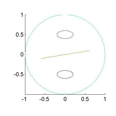
Here is an example of solving a two-dimensional boundary value problem using QMG. This is test file test7.m in the Matlab example directory. The Tcl/Tk example test7.tcl is similar, except it does not invoke the finite-element solver. The domain is a circle with two elliptic holes and one slit (an internal boundary). The boundary conditions are u=1 on one hole, u=2 on the other hole, and du/dn=0 (insulated) on the exterior and on the slit. First, here is script file for this test.

%% QMG 2.0 test 7: a circle with two elliptic holes and a slit.

echo on

global interactive
%% Make an approximation to a circle using 6 Bezier cubic arcs.

numseg = 6;
[verts, scrap] = gm_circ_approx(0, 2*pi, numseg);

[numvert,scrap] = size(verts);
verts = verts(1:3*numseg,:);
codes = kron(ones(numseg,1),[2;3;3]);
codes(1) = 0;

c0 = gm_cpoly(verts,codes);

%% Make two elliptic holes.

hole1 = gmapply([.2, 0, 0; 0,.1,-.5], c0);
c = gmcavity(c0,hole1);
hole2 = gmapply([.2, 0, 0; 0, .1, .5], c0);
c = gmcavity(c,hole2);

%% Make a slit by modifying the brep directly.


%% Insert two new control points at (-.6,-.1) and (.6,.1).
[scrap,numcp] = size(c{4});

c{4}(:,numcp:numcp+1) = [.6,-.6;.1,-.1];

%% Insert two new vertices at these points.

[scrap,numv] = size(c{5});

c{5}(:,numv:numv+1) = {
'newv1','newv2'
 {}, {}
 {}, {}
 {}, {}
{'vertex';[];numcp},{'vertex';[];numcp+1}
};

%% Insert a new edge connecting those vertices.

[scrap,nume] = size(c{6});

c{6}(:,nume) = {
'newe1'
{}
{'newv1','newv2'}
{}
{'bezier_curve';1;[numcp,numcp+1]}
};

%% Insert the new edge as a repeated boundary of the region.

oldbsize = length(c{7}{2,0}); 
c{7}{2,0}{oldbsize} = 'newe1';
c{7}{2,0}{oldbsize+1} = 'newe1';


c_color = gmrndcolor(c);

if length(interactive) > 0
  gmviz(c_color), gmshowcolor(c_color)
end

%% generate a mesh.  Elements of size about .2.

show = 0;
if length(interactive) > 0
  show = 1;
end

m = gmmeshgen(c_color,'size','(const .2)', 'show', show);


%% Display the mesh
if length(interactive) > 0
  gmviz(m)
end

[c_color2, m2] = gmdouble(c_color, {'*'}, m);

%% Check the mesh.

gmchecktri(c_color2,m2);


%% Default neumann BC du/dn=0 on all faces except the two
%% holes that get Dirichlet conditions.

for j = 0 : nume
  if length(findstr('cav1',double(c_color2{6}{0,j})))
    [npv,scrap] = size(c_color2{6}(1,j));
    c_color2{6}{1,j}(:,npv) = {'bc'; '(d (const 1))'};
  end
  if length(findstr('cav2',double(c_color2{6}{0,j})))
    [npv,scrap] = size(c_color2{6}(1,j));
    c_color2{6}{1,j}(:,npv) = {'bc'; '(d (const 2))'};
  end
end

u = gmfem(c_color2, m2);

if length(interactive) > 0
  gmplot(m2, u)
end

global aspprod
global meshsizesum

if length(aspprod) > 0
  aspprod = aspprod * asp;
  [scrap,numvtx] = size(m2{4});
  meshsizesum = meshsizesum + numvtx;
end

Maximum aspect ratio =        19.1017 achieved in
simplex #668 of topological entity mregion (2:0) which has vertices 52 372 388 
Maximum global side length =  0.206452
Minimum global altitude =     0.00212975
Number of nodes = 409 number of elements = 706

The brep produced by this mfile is illustrated in the following figure. The edges have been colored so that green corresponds to the insulated faces, red to the u=2 boundary condition, and blue to the u=1 boundary condition.

The mesh produced by the mesh generator is depicted in the following figure.

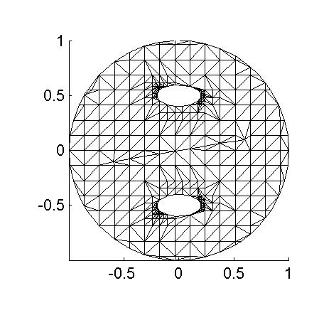
As seen from the above trace, the worst aspect ratio occurring in this mesh is about 19. It is obvious from looking at this mesh that the mesh generator could do better in the sense that there are nodes that could be locally displaced to improve the overall quality of the mesh. We have not yet implemented any heuristic improvement techniques.

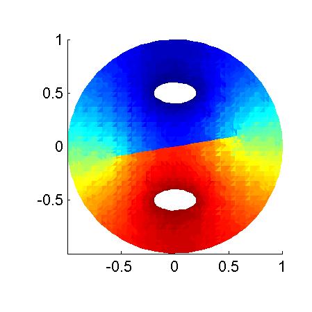
Finally, the color plot of the finite-element solution with mixed boundary conditions looks like this.

A 3-dimensional example

The mesh generator required 121 seconds on this example (Pentium Pro 166MHz). The properties of the resulting mesh are:

Maximum aspect ratio =        72.4505 achieved in
simplex #1190 of topological entity hexnutcrack (3:0) which has vertices 3 351 489 493 
Maximum global side length =  0.780871
Minimum global altitude =     0.00121479
Number of nodes = 807 number of elements = 3403

The brep used for this test was rendered in VRML by a call to gmviz function. You can see the object now if you have a VRML viewer installed in your browser. Two renderings are available: in the first rendering, the outer faces are shown, but they hide the internal boundary. In the second rendering, one of the outer surfaces has been made transparent using the statement:

gmset hexobj2 [gm_addpropval $hexobj {s_top} {color} {{(1 0 0 0)}}]

1. VRML rendering with all outer boundaries visible.
2. VRML rendering with one outer boundary invisible and internal boundary visible.

This documentation is written by Stephen A. Vavasis and is copyright ©1999 by Cornell University. Permission to reproduce this documentation is granted provided this notice remains attached. There is no warranty of any kind on this software or its documentation. See the accompanying file 'copyright' for a full statement of the copyright.