From the point of view of software development, the three most difficult aspects of finite element analysis are the geometric modeling tools, the mesh generator, and the finite element system solver. The QMG package is intended to address geometric modeling and mesh generation in three dimensions. It also has an elementary finite element solver that solves the sparse matrix equation with Matlab's backslash operator.
The QMG package consists of approximately 60 separate functions. The user of QMG invokes the functions through a console interface. QMG does not have its own console interface; instead it relies on the scripting capabilities of other software packages. Currently QMG runs inside of two different scripting environments: Matlab 4.2 and Tcl/Tk.
Because it is difficult for a user to remember how 60 functions work, QMG also provides a suite of examples demonstrating the use of many of these functions, as well as a help utility ("help" in Matlab; "gmhelp" in Tcl/Tk) to get on-line documentation on the functions. In addition, there is a browser-based reference manual.
Although the interface to QMG is by typing in functions, it would be easy to extend QMG with a GUI control since both Matlab and Tcl/Tk have GUI-building commands. We may try to embed QMG in other scripting languages such as Visual Basic in the future.
All the QMG functions, except for the examples shipped with the software, begin with the prefix ``gm,'' which is short for ``geometry.'' Functions that begin with ``gm_'' are lower-level ``internal'' functions.
Matlab has a single data type, namely, matrices. Likewise, Tcl/Tk has a single data type, strings. Therefore, QMG encodes its C++ objects as gibberish-filled matrices for Matlab and gibberish-filled strings for Tcl/Tk. The user operates on these objects via the various functions in the package.
QMG can handle polyhedral objects only. A polyhedral object is one that can be constructed by a finite sequence of unions and intersections of halfspaces. (A non-polyhedral object can be approximated by a polyhedral object with many small facets. But there is a very significant penalty in terms of performance of the modeler and mesh generator for objects with many small facets.)
If you are familiar with mesh generation, here are some of the distinguishing features of the QMG mesh generator that may be different from mesh generators you have used previously. On the positive side,
A user of the QMG package typically has two tasks to accomplish:
The geometric model is typically constructed in QMG by calling some of the basic constructors, applying various transformations to the constructed objects, and then applying boolean operations (set union, set difference, etc) to the objects, yielding the final desired shape.
For three-dimensional geometric modeling, graphics are crucial. QMG uses VRML1.0 for 3D graphics, so you need to have a web-browser (presumably either Netscape or Internet Explorer) that can view VRML files. For more information about VRML, see the VRML repository. This site includes a list of free and commercial VRML viewers.
Finite element analysis is available only in the Matlab version of QMG (not the Tcl/Tk version). For the finite element analysis, the user must call the mesh generator, set up the desired boundary conditions, and call the solver program. The boundary conditions can be arbitrary Matlab functions. They are associated with faces of the domain as property-value pairs of the faces.
Here is an example of solving a two-dimensional boundary value problem using QMG. This is test file ``test1.m'' in the Matlab example directory. The Tcl/Tk example ``test1.tcl'' is similar, except it does not invoke the finite element solver. The domain is a regular polygon with two holes and one slit (an internal boundary). The boundary conditions are u=1 on one hole, u=0 on the other hole, and du/dn=0 (insulated) on the exterior and on the slit. First, here is script file for this test.
echo on

%% Construct an approximately circular region with a triangular hole,
%% a rectangular hole, and a slit.

p1 = gmpolygon(17);

if exist('interactive'),...
  pause, ...
end, ...

% Make the slit, a vertical line segment.
slit = gm_emptybrep(2);
% add an endpoint at (0,0.6)
slit = gm_addface(slit, 0, eye(2), [0,0.6], [0,0.6]);
% another endpoint at (0,-0.6);
slit = gm_addface(slit, 0, eye(2), [0,-.6], [0,-.6]);
% now the vertical segment that joins them
slit = gm_addface(slit, 1, [1,0], 0, [0,0]);
% Make the two points children of the the edge.
slit = gm_addsubface(slit, 1, 0, 1, 0, 0);
slit = gm_addsubface(slit, 1, 0, 1, 0, 1);
% subtract the slit from the polygon.

p2 = gmsubtract(p1,slit);


%% Make a triangle, shrink it, translate it, and make the triangular hole

tri = gmpolygon(3);
tri1 = gmapply(gmcompose(gmtranslate(.4, .4), gmdilate(.2,.2)), tri);
p3 = gmsubtract(p2, tri1);

if exist('interactive'), pause,end

%% Make a diamond hole

t1 = gmtranslate(-.3,0);
t2 = gmrotate(pi/6);
t3 = gmdilate(.1,.3);
rect1 = gmapply(gmcompose(t1,gmcompose(t2,t3)), gmpolygon(4));
domain = gmsubtract(p3, rect1);


%% See what we have.


if exist('interactive'), ...
  domaincolor = gmrndcolor(domain);, ...
  gmviz(domaincolor), gmshowcolor(domaincolor), ...
  pause, ...
end


%% Generate a mesh.  Specify 0.2 as the refinement level.

mesh = gmmeshgen(domain,'size','(const 0.2)');


%% Display the mesh
if exist('interactive'), ...
  gmviz(mesh,'w'), ...
  pause, ...
end

%% Double the internal boundary so that it becomes two
%% coincident faces.  The internal boundary is face 17.

[dom2, mesh2] = gmdoubleib(domain, mesh, 17);

%% Display the properties of the mesh

gmget(mesh2)
gmchecktri(dom2,mesh2);

% Put Neumann condition =0 on the outside and on the slit.
% This is the default so we don't have to do anything.


% Put Dir. condition 1 on the triangular hole.
for i = 19:21,...
  dom2 = gm_addpropval(dom2,1,i,'bc', '< d (const 1)>');,...
end

% Put Dir. condition 0 on the rectangular hole.

for i = 22:25,...
  dom2 = gm_addpropval(dom2,1,i,'bc', '<d (const 0)>');,...
end


%% Other faces, including the slit, default to Neumann condition
%% of 0, which means insulated.

%% Solve the boundary value problem.  Conductivity=1 everywhere assumed.

u = gmfem(dom2, mesh2);

%% Plot the FEM solution

if exist('interactive'), ...
  colormap(jet), ...
  gmplot(mesh2,u), ...
  colorbar, ...
end
The mesh generator on this example required approximately 3 seconds
on a Pentium. The function gmchecktri in the above script produced
the following output:
Maximum aspect ratio =        4.9373432904364190e+00 achieved in triangle 56
which has vertices
29 (-9.1659511770675800e-01 -3.5509084034696290e-01  )  source = 1:8
75 (-8.6948200629062260e-01 -2.1705399986619930e-01  )  source = 2:0
74 (-9.3318961320104380e-01 -3.1225550971436470e-01  )  source = 1:8
Maximum global side length =  1.9826983055430820e-01
Minimum global altitude =     2.7826395502520620e-02
The command gmget(mesh) in the above script produced the following output:
 Type =         simpcomplex
 EmbeddedDim =  2
 IntrinsicDim = 2
 NumVertices =  264
 NumSimplices = 431
 Vertices =     [ (264-by-2) ]
 SourceSpec =   [ (264-by-2) ]
 Simplices =    [ (431-by-3) ]
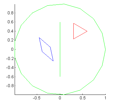
We now illustrate what this program produced
graphically. The original brep (``brep'' is the
term used for geometric objects in QMG) looks like this.
The edges have been colored so that green corresponds to the insulated
faces, red to the u=1 boundary condition, and blue to the
u=0 boundary condition.
The mesh produced by the mesh generator looks like this:
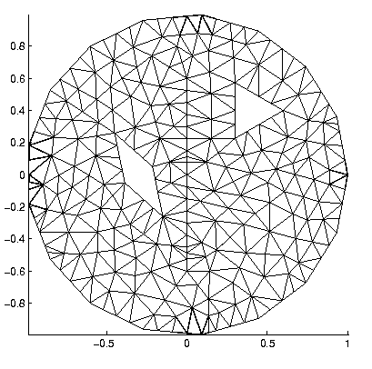
As seen from the above trace, the worst aspect ratio occurring in this mesh is about 4.9. It is obvious from looking at this mesh that the mesh generator could ``do better'' in the sense that there are nodes that could be locally displaced to improve the overall quality of the mesh. We have not yet implemented any heuristic improvement techniques.
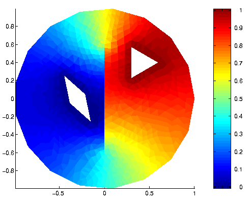
Finally, the color plot of the finite element solution with mixed boundary conditions looks like this.
## In this test, we'll construct a mesh for an interesting
## 3D shape, that is a tube with an annular pentagonal cross-section.
## Then we'll triangulate it.  We won't try a boundary value problem
## this time.

gmset base [gmpolygon 5]
gmset pyr [gmcone $base {0 0 2}]
gmset pyr1 [gmapply [gmtranslate 0 0 -.5] $pyr]
gmset pyr2 [gmsubtract $pyr $pyr1]
gmset pyr3 [gmapply [gmtranslate 0 0 1] $pyr]
gmset tubeobj [gmsubtract $pyr2 $pyr3]
gmget $tubeobj
gmset tubeobj [gmrndcolor $tubeobj]
if {[llength [info globals interactive]]} {
   gmviz $tubeobj
}

## Generate a coarse mesh for this object

gmset mesh [gmmeshgen $tubeobj size "(const 0.4)" showgui 0]

## Get information about the mesh.
gmget $mesh
gmchecktri $tubeobj $mesh
The results of the mesh generation is: a mesh with 2846 vertices
and 11540 tetrahedra was generated in 2 minutes and 48 seconds,
with a worst-case aspect ratio of about 270.
The brep used for this test was rendered in VRML by the above call to
gmviz
function. If you have VRML viewer plug-in
installed in your
web browser, you can click here to
view the object now.
This documentation is written by Stephen A. Vavasis and is copyright (c) 1996 by Cornell University. Permission to reproduce this documentation is granted provided this notice remains attached. There is no warranty of any kind on this software or its documentation. See the accompanying file 'Copyright' for a full statement of the copyright.
Back to the QMG 1.1 home page.
Stephen A. Vavasis, Computer Science Department, Cornell University, Ithaca, NY 14853, vavasis@cs.cornell.edu