CS 567
Assignment #4: Interactive Smoke Control
Due date: End of course (date
TBD).
In this fourth and final assignment
you defy the laws of physics and perform numerical magic by controlling
smoke to match target keyframes of your choosing. The approach we will
take is based on the SIGGRAPH 2004 paper by [Fattal
and Lischinski 2004]; Graphbib
page; ACM
Digital Library link (with SIGGRAPH presentation).
Your implementation should run interactively
for several nontrivial examples.
Starter Code (cs567.smoke):
This project has significant Java starter code, primarily to support
smoke simulation based on [Stam 1999; Fedkiw et al. 2001], OpenGL
rendering and a skeleton code for smoke control to
get you started. It is available here,
with online Javadoc
documentation here. In this assignment,
you will modify
this package as needed and however you like. Things you might want to
tinker with are simulation parameters, mouse/keyboard controls,
exception handling for neural input
device, etc.
- Smoke is
the main()
access point. It accepts image keyframes as input on the commandline.
You'll also find all keyboard and mouse controls in this
object; a summary of default key assignments is as follows:
- SPACE : toggles simulation.
- 'r' : Resets simulations, and pauses it.
- 'e' : Export frames toggle.
- FluidSolver:
This class is the basic fluid solver based on [Stam 1999; Fedkiw et al.
2001] and is a modified version of this "Stable Fluids" applet
by Alexander McKenzie (Caltech Multi-Res Modeling
Group), which is similar to Stam's GDC03 C implementation here.
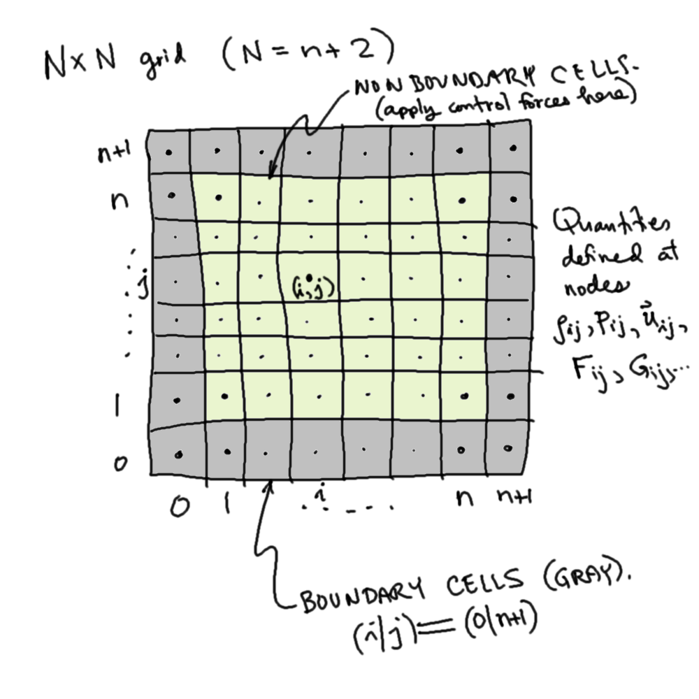
This basic solver will get you off on your way to controlling smoke,
but it's not ideal. Although the MAC grid is preferrable numerically, a
simple easy-to-understand grid definition is used in
which all values (velocity, pressure, density) are defined at the same
grid point--see this illustration. This
should make your coding
slightly easier.
- Constants: Useful
constants including grid
resolution, and forcing parameters are gathered in Constants
for your
tweaking convenience.
- Test Images: A variety of test
images are included in the "code/images" subdirectory. Add your
own
images! You will be able to easily use any image loadable via the
ImageIO library,
and they will be automatically sized, resampled to the
resolution specified in Constants,
and converted to grayscale.
- Software
Dependencies:
As before, the starter code will compile and run using JDK 1.5 or
later. I
recommend you get Sun's latest JDK here. In
addition to Java the starter code also uses JOGL/OpenGL and Vecmath
familiar from previous assignments. Although you're welcome to
modify the OpenGL portion of the assignment, it is not necessary to
complete it.
- Performance
Profiling: In addition to timing your broad and narrow phase
collision times, you can use the "java
-Xprof ..." option to help identify and remove program
bottlenecks (currently used in r.bat).
Assignment Steps: Your smoke solver
works out of the box. Here
are the steps and issues you need to address to control smoke---most of
which involve modifying the FluidSolver and SmokeControlForces
objects:
- Driving force: Modify
the skeleton code in SmokeKeyframe
and SmokeControlForces.getDrivingForce(...)
to implement the driving force term. First, since the
ratio of the gradient of the blurred goal density to the blurred goal
density, or (GRAD rhoGoalBlur)/rhoGoalBlur, does not change over time,
you can compute it once and for all in the constructor of the SmokeKeyframe--fill
in this code. Second, wire in the force in SmokeControlForces.getDrivingForce(...).
The driving force amplitude is controlled by Constants.V_f.
The drag or damping force, Constants.V_d
* u, is already implemented
for you in FluidSolver.velocitySolver().
- Gathering force:
Implement the smoke gathering force in SmokeControlForces.getGatheringRate(...)
using the discretization discussed in class, i.e., evaluate
the effective diffusion coefficient and gradients on cell edges, then
evaluate the divergence of the flux (=diffusion coeff * gradient) at
the cell center using the edge-based values.
- Visualization: Instead
of drawing the density field, try drawing other fields using a keyboard
control. Drawing the smoke control forces will help you understand what
your many parameters, such as blurring, are actually doing.
- Smoke preservation: You'll
notice that due to numerical dissipation the smoke tends to decay over
time, and therefore it can not match keyframes. This was one of the
motivations for the particular CFD solver used in [Fattal and
Lischinski 2004] but something you'll have to make the best of.
Mass preservation was also discussed in [Treuille et al. 2003].
Experiment with different normalization schemes that help match the
overall keyframe density norm. Be careful not to change the normal too
quickly or it may introduce artifacts, e.g., when changing
keyframes. Also simple scaling of the density field can produce
other artifacts... see what you can do to make it work.
- Stability: By this point
you should notice that the simulator is not always stable due to the
explicit integration of smoke control forces, and associated time-step
restriction. Also, reducing the smoke diffusion rate, Constants.SMOKE_DIFFUSION,
to zero can lead to artifacts. Experiment with stability for different
time steps, grid resolutions, and various parameter settings to
understand how to make your simulation more robust.
- Preconditioned Conjugate
Gradients (PCG) solver: One of bottlenecks and numerical
deficiencies of the starter code is that Gauss-Seidel relaxation is
used to solve the linear systems in FluidSolver.linearSolver(...).
This solver is used for both
the pressure Poisson equation solve, as well as to diffuse velocity or
smoke density if there are nonzero viscosity or smoke diffusion
coefficients, respectively. Use your previous PCG implementation
along with a suitable
preconditioner to make the simulation faster and better. There are many
possible preconditioners
including Jacobi, Gauss-Seidel, incomplete LU
(ILU), modified incomplete Cholesky (MIC), multigrid, etc. You might
also use an
FFT-based solver if you are willing to convert the problem to use
periodic boundary conditions (see the JGT article [Stam 2001]). For
example, this piece code
on Robert Bridson's
page implements MIC. The simplest choice is probably a Gauss-Seidel
relaxation--which you already have!
- Boundary conditions need
special care in your linear system solver. The starter code
approximates a Neumann BC with the normal derivative of pressure zero
at the boundary. Implement Neumann BCs correctly in your solver.
- Blur implementation bottleneck:
Another serious bottleneck of the skeleton implementation is
that the Gaussian blur (in Blur) is
approximated using iterative local-averaging, and is currently O(N^3)
for an N-by-N image and O(N) kernel radius. Although heavy
blurring is not required, the support of the effective blurring kernel
(Gaussian) must be large to avoid division by zero, and to produce
meaningful driving forces. Implement something
better (such as an FFT blur operator) to eliminate this bottleneck.
- Try one of the following if
you can: This is the final
project, and some of you may finish the above steps pretty
fast. In that case, you should try something a little more
challenging. Here are some ideas:
- 3D Extension:
Given a working 2D implementation, it's only a little more work to
convert the smoke solver to a full 3D implementation, e.g., replace I(i,j) with
I(i,j,k),
etc. See if you can blow smoke into the shape of a 3D solid
model, or make a ship sail through a smoke ring.
- MAC grids are better
than uniform grids, so give them a try.
- Improved advection: Try
implementing the improved advection with filtered cubic interpolation
from [Fedkiw et al. 2001] and see if that improves the quality of your
smoke.
- Implement [Fattal and
Lischinski 2004]: If you're more ambitious, go ahead and
implement the CFD solver described in the original paper, and see how
much it improves the quality of your animations.
- Internal boundaries can
be introduced with some modifications to your pressure solver, and can
let you model more interesting domains.
- Rigid objects can also
be introduced into the fluid with a modified linear solver, and some
coupling forces. Some related graphics papers you may find useful are [Carlson
et al. 2004], [Baxter
and Lin 2004], and [Guendelman
et al. 2005].
- Multiple smoke fields and
colors can be introduced as in [Fattal and Lischinski
2004]. Alternately, see if you can have smoke fields of RGB
colors that can transition between colors to match colored images.
- Fluid control: See if
you can control dyes in fluids with free surfaces similar to smoke.
Better still, try to control the shape of the fluid surface using
control forces. You can try implementing the FLIP scheme of [Zhu
and Bridson 2005] (consider this
starter code).
- Improved rendering: Consider
a ray-marching scheme (such as in [Fedkiw et al. 2001]) for improved
smoke rendering.
- Something else! Feel
free to talk to me about any other ideas you have.
- One
Creative
Smoke-Control Artifact!: One of the best parts of computer
animation is creative use of
mathematics and computer programming.
Create! Use your imagination to create
something
really interesting. Modify the starter code in any way you
want.
- Suggestion: Build a movie renderer: Load in a movie
image stack (using lazy loading) and use them as keyframes. See if you
can generate a class to render movies in smoke!
- Include videos of
your work, and also please
include one still image that represents your most interesting
scenario.
On
collaboration and academic integrity:
You are allowed to collaborate on the assignments to the extent of
formulating ideas as a group, and derivation of physical equations.
However, you must conduct your programming and write up completely on
your own, and understand what you are writing. Please also list the
names of everyone that you discussed the assignment with. (You
are expected to maintain the utmost level of academic integrity in the
course. Any violation of the code of academic integrity will be
penalized severely.)
Hand-in using CMS: Please
submit
a short write-up (detailing what you did, your findings, and who you
discussed the assignment with, etc.), as well as your Java
implementation, a creative simulation artifact(s), and videos of
anything you want me to see, etc.
References (see course homepage):
- J. Stam. Stable Fluids. In SIGGRAPH 99 Conference Proceedings,
Annual Conference Series , pages 121-128, August 1999.
- N. Foster and D. Metaxes. Modeling the Motion of a Hot, Turbulent
Gas. In SIGGRAPH 97 Conference Proceedings, Annual Conference Series ,
pages 181-188, August 1997.
- J. Stam, A Simple Fluid Solver based on the FFT. In Journal of
Graphics Tools, Volume 6, Number 2, pages 43-52, 2001.
- J. Stam, Real-Time Fluid Dynamics for Games. Proceedings of the
Game Developer Conference, March 2003.
- R. Fedkiw, J. Stam, and H. W. Jensen. Visual Simulation of Smoke.
In SIGGRAPH 2001 Conference Proceedings, Annual Conference Series ,
pages 15-22, August 2001.
Enjoy!!!
Copyright Doug James, April 2007.
