Can we prove that any given program works for all possible inputs? No, that question is undecidable. But can we develop a program for a given computable task so that we can prove that it works for all possible inputs? In principle, yes. In practice, this approach is too time-consuming to be applied to large programs. However, it is useful to look at how proofs of correctness can be constructed:
What is a proof? A completely convincing argument that something is true. For an argument to be completely convincing, it should be made up of small steps, each of which is obviously true. In fact, each step should be so simple and obvious that we could build a computer program to check the proof. Two ingredients are required:
A logic accomplishes these two goals.
The strategy for proving programs correct will be to convert programs and their specifications into a purely logical statement that is either true or false. If the statement is true, then the program is correct. But for our proofs to be truly convincing, we need a clear understanding of what a proof is.
Curiously, mathematicians did not really study the proofs that they were constructing until the 20th century. Once they did, they discovered that logic itself was a deep topic with many implications for the rest of mathematics.
We start with propositional logic, which is a logic built up from simple symbols representing propositions about some world. For our example, we will use the letters A, B, C, ... as propositional symbols. For example, these symbols might stand for various propositions:
It is not the job of propositional logic to assign meanings to these symbols. However, we use statements to the meanings of D and E to talk about the correctness of programs.
We define a grammar for propositions built up from these symbols. We use the letters P, Q, R to represent propositions (or formulas):
P,Q,R ::= ⊤                    (* true *)
        | ⊥                    (* false *)
        | A, B, C              (* propositional symbols *)
        | ¬P                   (* sugar for P⇒⊥ *)
        | P ∧ Q                (* "P and Q" (conjunction) *)
        | P ∨ Q                (* "P or Q" (disjunction) *)
        | P ⇒ Q               (* "P implies Q" (implication) *)
        | P ⇔ Q               (* "P if and only if Q" (double implication) *)
Note: On some browsers, on some operating systems, in some fonts, the symbol for conjunction (and) is rendered incorrectly as a small circle. It should look like an upside-down ∨. In this document, it will appear variously as ∧, ∧, or ∧.
The precedence of these forms decreases as we go down the list, so P ∧ Q ⇒ R is the same as (P ∧ Q) ⇒ R. One thing to watch out for is that ⇒ is right-associative (like →), so P ⇒ Q ⇒ R is the same as P ⇒ (Q ⇒ R). We will introduce parentheses as needed for clarity. We will use the notation for logical negation, but it is really just syntactic sugar for the implication P ⇒ ⊥. We also write P ⇔ Q as syntactic sugar for (P ⇒ Q) ∧ (Q ⇒ P), meaning that P and Q are logically equivalent.
This grammar defines the language of propositions. With suitable propositional symbols, we can express various interesting statements, for example:
In fact, all three of these propositions are logically equivalent, which we can determine without knowing about what finals and attendance mean.
In order to say whether a proposition is true or not, we need to understand what it means. The truth of a proposition sometimes depends on the state of the "world". For example, proposition D above is true in a world where x = 0 and y = 10, but not in a world in which x = y = 0. To understand the meaning of a proposition P, we need to know whether for each world, it is true. To do this, we only need to know whether P is true for each possible combination of truth or falsity of the propositional symbols A, B, C,... within it. For example, consider the proposition A ∧ B. This is true when both A and B are true, but otherwise false. We can draw a truth table that describes all four possible worlds compactly:
| ∧ | false | true | A |
|---|---|---|---|
| false | false | false | |
| true | false | true | |
| B |
This kind of table can also be used to describe the action of an operator like ∧ for a conjunction over general propositions P ∧ Q rather than over simple propositional symbols A and B. Here is a truth table for disjunction. Notice that in the case where both P and Q are true, we consider P ∨ Q to be true. The connective ∨ is inclusive rather than exclusive.
| ∨ | false | true | P |
|---|---|---|---|
| false | false | true | |
| true | true | true | |
| Q |
We can also create a truth table for negation ¬P:
| ¬ | false | true | P | |
|---|---|---|---|---|
| false | true | false |
Implication P ⇒ Q is tricky. The implication seems true if P is true and Q is true, and if P is false and Q is false. And the implication is clearly false if P is true and Q is false:
| ⇒ | false | true | P |
|---|---|---|---|
| false | true | false | |
| true | ? | true | |
| Q |
What about the case in which P is false and Q is true? In a sense we have no evidence about the implication as long as P is false. Logicians consider that in this case the assertion P ⇒ Q is true. Indeed, the proposition P ⇒ Q is considered vacuously true in the case where P is false, yielding this truth table:
| ⇒ | false | true | P |
|---|---|---|---|
| false | true | false | |
| true | true | true | |
| Q |
We can use truth tables like these to evaluate the truth of any propositions we want. For example, the truth table for (A ⇒ B) ∧ (B ⇒ A) is true in the places where both implications would be:
| ⇔ | false | true | A |
|---|---|---|---|
| false | true | false | |
| true | false | true | |
| B |
In fact, this means that A and B are logically equivalent, which we write as A iff B or A ⇔ B. If P ⇔ Q, then we can replace P with Q wherever it appears in a proposition, and vice versa, without changing the meaning of the proposition. This is very handy.
Another interesting case is the proposition (A ∧ B) ⇒ B. The truth table looks like this:
| (A∧B)⇒B | false | true | A |
|---|---|---|---|
| false | true | true | |
| true | true | true | |
| B |
In other words, the proposition (A ∧ B) ⇒ B is true regardless of what A and B stand for. In fact, it will be true if A and B are replaced with any propositions P and Q. We call such a proposition a tautology.
There are a number of useful tautologies, including the following:
| Associativity | (P ∧ Q) ∧ R ⇔ P ∧ (Q ∧ R) | (P ∨ Q) ∨ R ⇔ P ∨ (Q ∨ R) | |
| Symmetry | P ∧ Q ⇔ Q ∧ P | P ∨ Q ⇔ Q ∨ P | |
| Distributivity | P ∧ (Q ∨ R) ⇔ (P ∧ Q) ∨ (P ∧ R) | P ∨ (Q ∧ R) ⇔ (P ∨ Q) ∧ (P ∨ R) | |
| Idempotency | P ∧ P ⇔ P | P ∨ P ⇔ P | |
| DeMorgan's laws | ¬(P ∧ Q) ⇔ ¬P ∨ ¬Q | ¬(P ∨ Q) ⇔ ¬P ∧ ¬Q | |
| Negation | P ⇔ ¬¬P | (P ⇒ ⊥) ⇔ ¬P | (P ⇒ Q) ⇔ ¬P ∨ Q |
These can all be derived from the rules we will see shortly, but they are useful to know.
Notice that we can use DeMorgan's laws to turn ∧ into ∨, and use the equivalence P ⇒ Q ⇔ ¬P ∨ Q to turn ∨ into ⇒, and the equivalence (P ⇒ ⊥) ⇔ ¬P to get rid of negation. So we can express any proposition using just implication ⇒ and the false symbol ⊥!
Testing whether a proposition is a tautology by testing every possible truth assignment is expensive—there are exponentially many. We need a deductive system, which will allow us to construct proofs of tautologies in a step-by-step fashion.
The system we will use is known as natural deduction. The system consists of a set of rules of inference for deriving consequences from premises. One builds a proof tree whose root is the proposition to be proved and whose leaves are the initial assumptions or axioms (for proof trees, we usually draw the root at the bottom and the leaves at the top).
For example, one rule of our system is known as modus ponens. Intuitively, this says that if we know P is true, and we know that P implies Q, then we can conclude Q.
| (modus ponens) | ||||
The propositions above the line are called premises; the proposition below the line is the conclusion. Both the premises and the conclusion may contain metavariables (in this case, P and Q) representing arbitrary propositions. When an inference rule is used as part of a proof, the metavariables are replaced in a consistent way with the appropriate kind of object (in this case, propositions).
Most rules come in one of two flavors: introduction or elimination rules. Introduction rules introduce the use of a logical operator, and elimination rules eliminate it. Modus ponens is an elimination rule for ⇒. On the right-hand side of a rule, we often write the name of the rule. This is helpful when reading proofs. In this case, we have written (modus ponens). We could also have written (⇒-elim) to indicate that this is the elimination rule for ⇒.
Conjunction (∧) has an introduction rule and two elimination rules:
| (∧-intro) |
| (∧-elim-left) |
| (∧-elim-right) | ||||||||
The simplest introduction rule is the one for T. It is called "unit". Because it has no premises, this rule is an axiom: something that can start a proof.
| (unit) |
In natural deduction, to prove an implication of the form P ⇒ Q, we assume P, then reason under that assumption to try to derive Q. If we are successful, then we can conclude that P ⇒ Q.
In a proof, we are always allowed to introduce a new assumption P, then reason under that assumption. We must give the assumption a name; we have used the name x in the example below. Each distinct assumption must have a different name.
| (assum) |
Because it has no premises, this rule can also start a proof. It can be used as if the proposition P were proved. The name of the assumption is also indicated here.
However, you do not get to make assumptions for free! To get a complete proof, all assumptions must be eventually discharged. This is done in the implication introduction rule. This rule introduces an implication P ⇒ Q by discharging a prior assumption [x : P]. Intuitively, if Q can be proved under the assumption P, then the implication P ⇒ Q holds without any assumptions. We write x in the rule name to show which assumption is discharged. This rule and modus ponens are the introduction and elimination rules for implications.
| (⇒-intro/x) |
| (⇒-elim, modus ponens) | ||||||
A proof is valid only if every assumption is eventually discharged. This must happen in the proof tree below the assumption. The same assumption can be used more than once.
| (∨-intro-left) |
| (∨-intro-right) |
| (∨-elim) | |||||||||||
A negation ¬P can be considered an abbreviation for P ⇒ ⊥:
| (¬-intro) |
| (¬-elim) |
| (reductio ad absurdum, RAA/x) |
| (ex falso quodlibet, EFQ) | |||||
Reductio ad absurdum (RAA) is an interesting rule. It embodies proofs by contradiction. It says that if by assuming that P is false we can derive a contradiction, then P must be true. The assumption x is discharged in the application of this rule. This rule is present in classical logic but not in intuitionistic (constructive) logic. In intuitionistic logic, a proposition is not considered true simply because its negation is false.
Another classical tautology that is not intuitionistically valid is the the law of the excluded middle, P ∨ ¬P. We will take it as an axiom in our system. The Latin name for this rule is tertium non datur, but we will call it magic.
| (magic) |
A proof of proposition P in natural deduction starts from axioms and assumptions and derives P with all assumptions discharged. Every step in the proof is an instance of an inference rule with metavariables substituted consistently with expressions of the appropriate syntactic class.
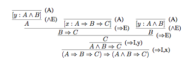
For example, here is a proof of the proposition (A ⇒ B ⇒ C) ⇒ (A ∧ B ⇒ C).
The final step in the proof is to derive (A ⇒ B ⇒ C) ⇒ (A ∧ B ⇒ C) from (A ∧ B ⇒ C), which is done using the rule (⇒-intro), discharging the assumption [x : A ⇒ B ⇒ C]. To see how this rule generates the proof step, substitute for the metavariables P, Q, x in the rule as follows: P = (A ⇒ B ⇒ C), Q = (A ∧ B ⇒ C), and x = x. The immediately previous step uses the same rule, but with a different substitution: P = A ∧ B, Q = C, x = y.
The proof tree for this example has the following form, with the proved proposition at the root and axioms and assumptions at the leaves.

A proposition that has a complete proof in a deductive system is called a theorem of that system.
A measure of a deductive system's power is whether it is powerful enough to prove all true statements. A deductive system is said to be complete if all true statements are theorems (have proofs in the system). For propositional logic and natural deduction, this means that all tautologies must have natural deduction proofs. Conversely, a deductive system is called sound if all theorems are true. The proof rules we have given above are in fact sound and complete for propositional logic: every theorem is a tautology, and every tautology is a theorem.
Finding a proof for a given tautology can be difficult. But once the proof is found, checking that it is indeed a proof is completely mechanical, requiring no intelligence or insight whatsoever. It is therefore a very strong argument that the thing proved is in fact true.
We can also make writing proofs less tedious by adding more rules that provide reasoning shortcuts. These rules are sound if there is a way to convert a proof using them into a proof using the original rules. Such added rules are called admissible.