Problem Set 2: Folding and Datatypes
Due Monday 9/21/09 11:59pm
Important notes about grading:
- Compile errors: All programs that you submit must compile.
Programs that do not compile will probably
receive an automatic zero. If you are having trouble getting your
assignment to compile, please visit consulting hours. If you run out of
time, it is better to comment out the parts that do not compile and
hand in a file that compiles, rather than handing in a more complete
file that does not compile.
- Missing functions: We will be using an automatic grading
script, so it is crucial that you name
your functions and order their arguments according to the problem set
instructions, and that you place the functions in the correct files. Otherwise
you may not receive credit for a function properly written.
- Code style: Please pay attention to style. Refer
to the CS 3110 style guide and lecture notes. Ugly code that is functionally
correct may still lose points. Take the extra time to think through
the problems and find the most elegant solutions before coding them up.
- Wrong versions: Please double-check that you are submitting the correct versions of your files to CMS.
The excuse, "I had it all done, but I accidentally submitted the wrong files" will not be accepted.
Part 1: List Folding (35 points)
Folding is one of the most
useful tools in functional programming and you will certainly use it
many times over the course of the semester. The following exercises
are designed to get you comfortable with folding to do useful
computations on lists. Note: All of these functions can be written
without folding, but the point of the exercise is to get used to
folding, so every function must include either List.fold_left or
List.fold_right. For full credit, do not use the rec keyword.
- Write a function
max2 : int list -> int that
returns the second-greatest value in the list.
Example: max2 [1110; 3110; 2110; 2800; 4820] = 3110.
Do not sort the list. Raise an exception with a helpful message if the list is too short.
Note: there may be duplicates in the list, and the second-greatest
value may be the same as the greatest, in which case you should return it.
I.e., the result should be the same as if you sorted the list in descending
order and took the second element.
- The powerset of a set A is the set of all subsets of
A. Write a function
powerset : 'a list -> 'a list list
such that powerset s returns the powerset of
s, interpreting lists as unordered sets.
You may assume there are no duplicate elements in
s. More precisely, for every subset
T of the elements in s, there is a list in
powerset s that contains exactly the elements of
T.
Example: powerset [1; 2; 3] = [[]; [1];
[2]; [3]; [1; 2]; [1; 3]; [2; 3]; [1; 2; 3]].
The order of the sublists you return and the order of the elements in each
sublist do not matter. Your program may return the elements in a different order
from the example above.
-
Write a function
inverted_index : string list list -> (string * int list) list.
The nth element of the input list is the set of keywords that appear on the nth page of a book.
For each keyword in the book, inverted_index gives a list of pages on which it appeared.
For full credit:
- The keywords should appear in lexicographical (dictionary) order.
- For each keyword, the page numbers should appear in ascending order.
- For each keyword, there are no duplicate page numbers, even if the keyword appeared multiple times on a page.
Example: inverted_index [["ocaml"; "is"; "is"; "fun"]; ["because"; "fun"; "is"; "a"; "keyword"]]
= [("a", [1]); ("because", [1]); ("fun", [0; 1]); ("is", [0; 1]); ("keyword", [1]); ("ocaml", [0])]
Part 2: Symbolic Differentiation (35 points)
In the Summer of 1958, John McCarthy (recipient of the Turing Award in
1971) made a major contribution to the field of programming
languages. With the objective of writing a program that performed
symbolic differentiation of algebraic expressions, he noticed that
some features that would have helped him to accomplish this task were
absent in the programming languages of that time. This led him to the
invention of LISP (published in Communications of the ACM in 1960) and
other ideas, such as list processing (the name Lisp derives from "List
Processing"), recursion and garbage collection, which are essential to
modern programming languages, including Java. Nowadays, symbolic
differentiation of algebraic expressions is a task that can be
conveniently accomplished with modern mathematical packages, such as
Mathematica and Maple.
The objective of this part is to build a language that can
differentiate and evaluate symbolically represented mathematical
expressions that are functions of a single variable x. Symbolic
expressions consist of numbers, variables, and standard functions
(plus, minus, times, divide, sin, cos, etc). To get
you started, we have provided the datatype that defines the
abstract syntax for such expressions.
(* abstract syntax tree *)
(* Binary Operators *)
type bop = Add | Sub | Mul | Div | Pow

(* Unary Operators *)
type uop = Sin | Cos | Ln | Neg

type expr = Num of float
          | Var
          | BinOp of bop * expr * expr
          | UnOp of uop * expr
This datatype provides an internal representation of an expression
that the user might type in. The constructor
Var represents the single variable x, and
UnOp (Ln, Var) represents the natural logarithm of x.
Neg refers to unary negation and is denoted by the symbol ~.
(the symbol - is only used for subtraction). The meaning of the others
should be clear.
Mathematical expressions can be constructed using the
constructors in the above datatype definition. For example, the expression
x^2 + sin(~x) would be
represented internally as:
BinOp (Add, BinOp (Pow, Var, Num 2.0), UnOp (Sin, UnOp (Neg, Var)))
This represents a tree in which nodes are the type constructors
and the children of each node are an operator and the
arguments of that operator. Such a tree is called an abstract
syntax tree (or AST for short).
For your
convenience, we have provided a function parse_expr which
translates a string in infix form (such as x^2 +
sin(~x)) into a value of type expr.
The parse_expr function
parses according to the standard precedence of operations, so
5 + x * 8 will be read as
5 + (x * 8). We have also provided two functions
to_string and to_string_smart
that print expressions in a readable form
using infix notation. The former produces a fully-parenthesized
expression so you can see how the parser parsed the expression,
whereas the latter omits unnecessary parentheses.
# let e = parse_expr "x^2 + sin(~x)";;
val e : Expression.expr =
  BinOp (Add, BinOp (Pow, Var, Num 2.), UnOp (Sin, UnOp (Neg, Var)))
# to_string e;;
- : string = "((x^2.)+(sin((~(x)))))"
# to_string_smart e;;
- : string = "x^2.+sin(~(x))"
- Write a function
fold_expr : (expr -> 'a) -> (uop -> 'a
-> 'a) -> (bop -> 'a -> 'a -> 'a) -> expr -> 'a
such that
fold_expr atom unary binary expr performs a postorder traversal of
expr. During the traversal, it applies atom :
expr -> 'a to every leaf node (i.e. Var or
Num). It applies unary : uop -> 'a -> 'a
to every unary expression. The first argument to unary
is the unary operator and the second is the result of applying
fold_expr recursively to that expression's operand. Finally,
fold_expr applies binary : bop -> 'a -> 'a ->
'a to every binary expression. The arguments to
binary are the binary operator and the results of
recursively applying fold_expr to the left and right operands.
For example, here is a function that uses fold_expr to
determine whether the given expression contains a variable.
let contains_var : expr -> bool =
  let atom = function
      Var -> true
    | _ -> false in
  let unary op x = x in
  let binary op l r = l || r in
    fold_expr atom unary binary
- Using
fold_expr, write a function eval : float
-> expr -> float such that eval x e evaluates
e, setting Var equal to the value
x.
Example: eval 2.0 (BinOp (Add, Num 2.0, Var)) = 4.0.
- Using
fold_expr, write a function derivative :
expr -> expr that returns the derivative of an expression with
respect to Var. The expression it returns need not be
simplified.
Example: derivative (BinOp (Pow, Var, Num 2.0))
= BinOp (Mul, Num 2., BinOp (Mul, Num 1., BinOp (Pow, Var, BinOp (Sub,
Num 2., Num 1.))))
When implementing this function, recall the
chain rule from your freshman calculus course:

This rule tells how to form the derivative of the composition of two functions if
we know the derivatives of the two functions.
With the help of this rule, we can write the derivatives
for all the operators in our language:
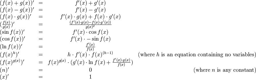
There are two cases provided for calculating the derivative of f(x) ^ g(x),
one for where g(x) = h does not contain any variables, and one for the general case.
The first is a special case of the second, but it is useful to treat them separately, because when the first case applies, the second case produces
unnecessarily complicated expressions.
Part 3: Quadtrees (30 points)
A quadtree is a
data structure that supports searching for objects located in a
two-dimensional space. To avoid spending storage space on empty
regions, quadtrees adaptively divide 2D space. Quadtrees are heavily
used in graphics and simulation applications for tasks such as quickly
finding all objects near a given location and detecting
collisions.
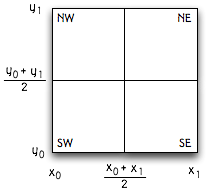
There are many variations on
quadtrees specialized for different applications. For this problem
set, we'll use a variation in which each node represents a
rectangular region of space parameterized by x and y coordinates: all the space between x
coordinates x0 and x1
and between y
coordinates y0
and y1.
A leaf node contains some (possibly empty) set of objects that are
all located at the same point (x, y),
which must lie within the leaf's rectangle. A
non-leaf node has four children, each covering one quarter of the
parent node's rectangle, as shown in this picture:
To insert an object at coordinates (x,y), we traverse the quadtree starting
from the top node and walk down through the appropriate sequence of
child nodes that contain the point (x,y) until we reach a leaf node. This
figure depicts the quadtree nodes that we visited in the process of
inserting an object located at the black dot.
If the object to be inserted is at the same point as the other objects
at that leaf, we can just add it to the leaf's list of objects.
Otherwise we must split the leaf into quadrants.
We have defined the quadtree datatype and documented the
Quadtree module for you. In our implementation, an empty
leaf is represented by the datatype constructor Nil and a
non-empty leaf with the constructor Leaf. Non-leaf nodes
are represented with the datatype constructor Split.
Your task is to finish implementing two functions insert
and fold_rect, following the specifications in
quadtree.ml. Neither function should require much code. In our
solution, the two functions together are less than 30 lines of code.
Make use of the functions in the Rect module and the
helper functions in the Quadtree module.
We have provided you with a dataset (us-places.txt)
containing the names of thousands of places in the US along with their
latitude and longitudes. The purpose of this dataset is to help you
test your quadtree. You can load it using the City
module.
Karma
This part contains two karma problems that are not
required for the problem set. It is included as an avenue for
students to further explore issues associated with symbolic
differentiation and the representation of expressions. We will grade
them if you do them; you will receive no points but plenty of
good karma if you do well.
- Implement a function
City.nearby_cities such that
City.nearby_cities qt lat long r returns the names of all
of the cities in the quadtree qt that are within a
distance r of (lat, long).
For the distance function, just use the Euclidean distance, i.e.
the distance from (lat1, long1) to (lat2, long2) is simply
sqrt((lat1 - lat2)^2 + (long1 - long2)^2). You do not
need to account for the curvature of the Earth.
- Consider the application
of the derivative function to the expression
x^2+sin(2*x)
and the corresponding output:
# to_string_smart (derivative (parse_expr "x^2 + sin(2*x)"));;
- : string = "2.*1.*x^(2.-1.)+cos(2.*x)*(0.*x+2.*1.)"
This expression appears unnecessarily complicated.
However, it can be
simplified to 2*x+cos(2*x)*2 using various elementary
simplifications.
Two basic types of reductions can be performed.
The first and more obvious is to carry out operations
that we have a simplified form for.
One such simplification is carrying out arithmetic on constants: if we
have two constants that are being added, multiplied, etc.,
we can reduce them to the result.
Additionally, some operations have predefined results for certain
constants or when the operands are equal.
We could perform reductions for other values of ln, sin, and cos,
but it is not advisable to do so, as there can be a loss of precision.
We expect you to implement the following simplifying reductions:
- All arithmetic on constants should be carried out
- 0 + f = f
- f + 0 = f
- 0 − f = ~f
- f − 0 = f
- 0 / f = 0
- f / 1 = f
- 1 * f = f
- f * 1 = f
- 0 * f = 0
- f * 0 = 0
- f ^ 0 = 1
- 0 ^ f = 0 (other than 0 ^ 0, which is defined as 1)
- f ^ 1 = f
- ln(1) = 0
- sin(0) = 0
- cos(0) = 1
- ~0 = 0
- f + f = 2 * f
- f * f = f ^ 2
- f − f = 0
- f / f = 1
The second type of reduction is to group similar operations and move negations
to the outside; there are few real simplifications we can do when negation is involved,
but many we can do with the other operations. In and of themselves, these reductions
don't do very much; their true power is enabling other reductions. One of these
reductions is to transform all negative constants into the unary operator negation applied
to a positive constant. For example, consider (-1)*f.
With the above reduction, it
will be converted to (~1)*f, and then other reductions will
will convert it to ~(1*f) and then ~f. Note that we write -n for an actual negative
constant (i.e., Num (-5.0),
and ~n for the unary operator negation applied to something (i.e., UnOp (Neg, Num 5.0)).
We expect you to implement the following reductions:
- −n = ~n
- ~~f = f
- ~f + g = g − f
- f + (~g) = f − g
- f − (~g) = f + g
- ~f − g = ~(f + g)
- (~f) * g = ~(f * g)
- f * (~g) = ~(f * g)
- (f/g) * h = (f * h) / g
- f * (g/h) = (f * g) / h
- (~f) / g = ~(f / g)
- f / (~g) = ~(f / g)
- (f / g) / h = f / (g * h)
- f / (g / h) = (f * h) / g
- f ^ (~g) = 1 / (f ^ g)
- (f ^ g) ^ h = f ^ (g * h)
It is worth noting that applying one reduction to an expression may
enable another. One consequence of this is that subexpressions
should be reduced first. For example, to fully reduce
x + (sin(x)−sin(x)), you should first reduce sin(x)−sin(x) to 0,
transforming the expression to x + 0, then reduce x + 0 to x.
Furthermore, note that as in the (~1)*f example above, you may need to apply multiple
reduction rules in sequence to an expression.
Your task is to implement a function reduce : expr -> expr that
performs all these reductions.