Topics:
Previously we saw one algorithm for exploring the nodes (vertices) of a graph starting from a source node: breadth-first search (BFS). BFS explores a graph in the order of the minimum path length from the source node to the given node. Recall what the pseudo-code looks like:
// let s be the source node
q = new Queue()
mark s visited
q.push(s)
while q not empty {
    Vertex v = q.pop()
    for each successor v' of v {
	if v' not visited {
	    mark v' visited
	    q.push(v')
	}
    }
}
When q is a first-in, first-out (FIFO) queue, we get
breadth-first search. All the nodes on the queue have a minimum path length
within one of each other. In general, there is a set of nodes to be
popped off, at some distance k from the source, and another set
of elements, later on the queue, at distance k+1. Every time a new
node is pushed onto the queue, it is at distance k+1 until all the
nodes at distance k are gone, and k then goes up by one.
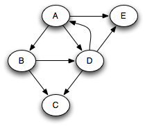
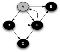
Suppose that we run this algorithm on the following graph, assuming that successors are visited in alphabetic order from any given node: :
In that case, we get the following queue states, where each node is annotated by its minimum distance from the source node A. Note that we're pushing onto the top of the queue and popping from the bottom.
A 0   E 1   C 2
      D 1   E 1   C 2
      B 1   D 1   E 1   C 2
time→
So we end up popping the nodes in distance order: A, B, D, E, C. When a queue is used in this way, it is known as a worklist; it keeps track of work left to be done.
What if we were to replace the FIFO queue with a LIFO stack? In that case we get a completely different order of traversal:
A 0   E 1   D 1   C 2   B 1
      D 1   B 1   B 1
      B 1
time→
With a stack, the search will proceed from a given node as far as it can before backtracking and considering other nodes on the stack. For example, the node B had to wait until all nodes reachable from D and E were considered. This is a depth-first search.
A more standard way of writing depth-first search is as a recursive function,
using the program stack as the stack above. To help us understand how the
algorithm works, we will imagine that every node can be either white, gray,
or black. Nodes that have never been visited are white. Vertices are colored
gray when they are first reached, and colored black when all nodes reachable
from them have been found. The colors will not affect the algorithm; they are
just to help understanding. We start with every node white and apply the
function DFS_visit to the starting node:
DFS_visit(Vertex v) {
    mark v visited
    set color of v to gray
    for each successor v' of v {
	if v' not yet visited {
	    DFS_visit(v')
	}
    }
    set color of v to black
}
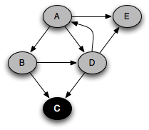
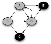
You can think of this as a person walking through the graph following arrows and never visiting a node twice except when backtracking when a dead end is reached. Running this code on the graph above yields the following graph colorings in sequence:

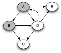


Notice that at any given time there is a single path of gray nodes
leading from the starting node and leading to the current node
v. This path corresponds to the stack in the earlier
implementation, although the nodes end up being visited in a different
order because the children of a node are considered in the opposite order
by the two depth-first searches.
The amount of state that the algorithm is mantaining is proportional to the size of this path from the root, which makes DFS rather different from BFS, where the amount of state (the queue size) corresponds to the size of the perimeter of nodes at distance k from the starting node. In both algorithms the amount of state can be O(|V|). For DFS this happens when searching a linked list. For BFS this happens when searching a graph with a lot of branching, such as a binary tree, because there are 2k nodes at distance k from the root. On a balanced binary tree, DFS maintains state proportional to the height of the tree, or O(log |V|). Often the graphs that we want to search are more like trees than linked lists, and so DFS tends to run faster.
There can be at most |V| calls to DFS_visit. And the body of the loop on successors can be executed at most |E| times. So the asymptotic performance of DFS is O(|V| + |E|), just like for breadth-first search.
If we want to search the whole graph, then a single recursive traversal may not suffice. For example, if we start a traversal with node C, we would miss all the rest of the nodes in the graph. To do a depth-first search of an entire graph, we call DFS_visit on an arbitrary unvisited node, and repeat until every node has been visited.
We can classify the various edges of the graph based on the color of the node reached when the algorithm follows the edge. Here is the same graph with the edges colored to show their classification. Note that the way we classify the edges depends on what node we start from and in what order the algorithm happens to select successors to visit.

When the destination node of a followed edge is white, this is when the algorithm performs a recursive call. These edges are called tree edges. The graph looks different in this picture because the nodes have been moved to make all the tree edges go downward. The nodes of the graph plus the tree edges always form a tree. In fact, the tree edges also show the precise sequence of recursive calls performed during the traversal. This is called the call tree of the program, and any program has a call tree.
When the destination of the followed edge is gray, it is a back edge, shown in red. Because there is only a single path of gray nodes, a back edge is looping back to an earlier gray node, creating a cycle. A graph has a cycle if and only if it contains a back edge when traversed from some node.
When the destination of the followed edge is colored black, it is a forward edge or a cross edge. If there is a path from the source node to the destination node through tree edges, it is a forward edge. Otherwise, it is a cross edge.
It is often useful to know whether a graph has cycles. To detect whether a graph has cycles, we perform a depth-first search of the entire graph. If a back edge is found during any traversal, the graph contains a cycle. If all nodes have been visited and no back edge has been found, the graph is acyclic.
One of the most useful algorithms on graphs is topological sort, in which the nodes of an acyclic graph are placed in an order consistent with the edges of the graph. This is useful when you need to order a set of elements where some elements have no ordering constraint relative to other elements. It is impossible to topologically sort a graph with a cycle in it.
For example, suppose you have a set of tasks to perform, but some tasks have to be done before other tasks can start. In what order should you perform the tasks? This problem can be solved by representing the tasks as node in a graph, where there is an edge from task 1 to task 2 if task 1 must be done before task 2. Then a topological sort of the graph will give an ordering in which task 1 precedes task 2. Obviously, to topologically sort a graph, it cannot have cycles. For example, if you were making lasagna, you might need to carry out tasks described by the following graph:

There is some flexibility about what order to do things in, but clearly we need to make the sauce before we assemble the lasagna. A topological sort will find some ordering that obeys this and the other ordering constraints.
Algorithm:
Perform a depth-first search over the entire graph, starting anew with an unvisited node if previous starting nodes did not visit every node. As each node is finished (colored black), put it on the head of an initially empty list. This clearly takes time linear in the size of the graph: O(|V| + |E|).
For example, in the traversal example above, we would get the ordering A, B, D, E, C, which can be seen by looking at the order in which nodes turn black. This ordering clearly is a topological sort of the graph.
Now, why does this work? The algorithm puts nodes onto the list in the reverse order in which they are finished. So the algorithm works as long as for every edge v→v', v' is finished later than v. Because the graph is acyclic, DFS only finds white and black nodes when traversing the graph. So when it follows the edge from v to v', it will either discover that v' is white or black. If v' is white, the algorithm will make a recursive call that will turn v' black before the current node, v, is turned black. And if it finds that v' is black, that node is already finished, yet v is not. So in either case, v' is finished before v.
Graphs need not be connected, although we have been drawing connected graphs thus far. It is entirely possible to have a graph in which there is no path from one node to another node, even following edges backward. For (weak) connectedness, we don't care which direction the edges go in, so we might as well consider an undirected graph. For example, the following undirected graph has three disconnected components.

The connected components problem is to determine how many connected components make up a graph, and to make it possible to find, for each node in the graph, which component it belongs to. For example, suppose that different components correspond to different jobs that need to be done, and there is an edge between two components if they need to be done on the same day. Then to find out what is the maximum number of days that can be used to carry all the jobs, we need to count the components.
Algorithm:
Perform a depth-first search over the graph. As each traversal starts, create a new component. All nodes reached during the traversal belong to that component. The number of traversals done during the depth-first search is the number of components. If the graph is directed, the DFS needs to follow both incoming and outgoing edges.
There is another version of this problem called the strongly connected components problem. Nodes are in the same strongly connected component if they can each be reached from each other. For directed graphs, there is a different between strongly connected and weakly connected components. The algorithm is more subtle, but again is a matter of using depth-first search.