2.5 Introduction to Probability

2.5.1 Random Variables and Events

A random variable is a variable with a range of possible values.

Examples:

• the duration of a CS664 lecture
• 
• 

Random variables (RVs) and be discrete (like x) or continuous (like y). To describe a random variable, you need some notion of the relative likelihood of the different possible values.

A sample assigns a RV one of its possible values, denoted by x=a.

An event is

1. a sample or
2. a conjunction, disjunction or negation of other events.

Examples:

• is a sample. It's also an event.
• is a sample. It's also an event.
• is an event.

2.5.2 Probability measures

A probability measure is a function that defines the probability of all different events.

Example:

The events		(x=2)	(x=3)	(x=4)
happen		¼	½	¼		of the time.

The numbers in the lower row are the probabilities.

More formally, a probability measure is a function P that satisfies the following axioms:

1. For any event A, P(A)>= 0
2. P(U)= 1, where U is the disjunction of all events.
3. If AB=0, then P(A+B)=P(A)+P(A)

With AB we denote that both events A and B are happening, and with A+B we denote the event A or B is happening. 0 denotes the impossible event, that is, 'AB=0' expresses that the events A and B are mutually exclusive. Condition 2 simply means that one of the events has to occur.

The probability of a sample ( y=a) for a continuous variable y has the probability P(y=a) = 0, even if the variable takes on this value quite often and should intuitively have a higher probability than the assignment of a value that is not even in the range of possible values.We will see the mathematical reasons for it in section 2.5.4.
Notice that the statement "a:P(y=a) = 0 is not a contradiction to the second condition because there are uncountably many events.

2.5.3 Distributions

A probability distribution F_x(a), also called cumulative density function is a function that associates each value a with the probability of the event (x<=a),

Example:

For a discrete RV x ,

For the above example, the probability distribution looks like

.

2.5.4 Probability density functions (pdf)

A probability density function f_y(a) maps each value to the derivative of F_x for that value,

that is, f_y(a) = d/da F_y(a).

Basic properties of a probability density function f_y are

Now let's try to understand better how probability, distributions and pdf's are related.

• First notice that .
  This follows directly from the definition of a pdf.
• Now remember from the last example that F_x(a) for a discrete variable x is given by .
  These two formulas are quite similar, but there is more going on than just the substitution of the integral by the summation: the probability density function f_y(a) does not return the probability of the event (y=a); remember that P(y=a)= 0, whereas f_y(a) can be non-zero.
• The equation also gives you an explanation why P(y=a)= 0 for continuous variables y: .

2.5.5 Probability mass functions (pmf)

There are no probability density functions for discrete variables because their probability distribution functions are also discrete and cannot be derived. The equivalent of a pdf for discrete variables is called probability mass function.

A probability mass function for a discrete RV x is a set of p_i's s.t.

for all i: p_i >= 0

for all i: p_i = P(x=i)

2.5.6 Expectation

The expectation value m is one of the fundamental quantities which characterize a random variable. The expectation value is also often called mean, average or first moment. It is usually denoted by E(x) or h, but there are also papers in which the notation <x> is used. The expectation value is defined as follows(the definition on the left is for continuous variables y, the one on the right for discrete variables):

.

The expectation for a function g(x) is defined by

.

You can see that the expectation value is just a weighted average of all values, where each possible value is weighted by the probability of its occurence. Another interpretation of the expectation is that if you consider the area below the pdf (the lower envelope of the pdf), the expectation value corresponds to the center of mass for this area.

Notice that the expectation inherits the property of linearity from the integral (or the summation, for that matter), that is

E(x+a*y)= E(x) + a*E(y).

This property allows very often a considerable simplification of the computation of the expectation value. We will see an example of this in section 2.5.7.

2.5.7 Variance and Standard Deviation

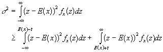
The variance of a random variable s² is another basic property and defined by s² =E( (x-h)² ), where h denotes E(x), as mentioned in the last paragraph.

It is also called the second central moment ¹.The quantity s is called standard deviation.

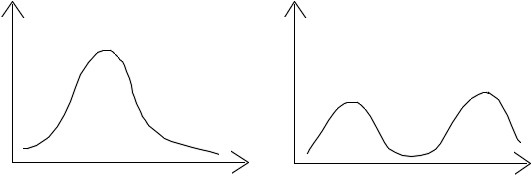
Variance and standard deviation measure the spread of a probability density function.
Example:

The pdf on the left has a lower variance and standard deviation than the pdf on the right.

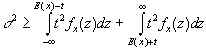
An easy transformation shows that

.

This formula is often used in practice to compute the variance.

It is conceivable to use different quantities to measure the center and spread of a pdf. Chebychev's theorem allows us however to make a rigorous argument why expectation and variance are actually a good way to describe probability density functions ².

2.5.8 Chebychev's Theorem

Chebychev's inequality

Let x be a RV with expectation m and (finite) variance s².

Then for all t >= 0,

.

Proof:

With t>0 we have

The second inequality holds because the integrand in the leftmost integration is always positive. By removing an integral of length 2t from the range of that integral, we do not increase the value of the integral. Inside the two integrals on the right-hand side of the above relation, it is always true that |z-E(x)|>=t. Therefore, we can safely replace [z-E(x)]² by t²:

.

We get Chebychev's inequality after we divide both sides by t² .q.e.d.

Now consider t = bs. Substitution yields

. Division by s leads to

.

The latter is usually read in the following way: 'The chance that x differs from m more than b standard deviations is below ". The interesting thing about Chebychev's inequality is that it holds independently of the actual distribution of x. There exist stronger theorems for RV's with special distributions.

2.5.9 Conditional Probability

Conditional probability deals with the probability of events whose likelihood is influenced by the (prior) occurence of other events.

Consider two events A and B. The conditional probability of B given A, written as P(B|A), is defined as

If A has no effect on B then P(B|A)= P(B). Therefore, P(AB)=P(A)*P(B). Events A and B for which this holds are called independent.

2.5.10 Probability, Statistics, Stochastic Methods and Randomized Algorithms

Finally, we want to clarify the use of four terms that often occur in the context of non-deterministic computer vision methods.

1. In probability, the relative frequency of certain events is known for a population and we ask for the probability of events for a subset of this population. Probability techniques are sound; the field is part of mathematics.
2. In statistics, the relative frequency of certain events is known for a subset of a population³ and you induce from that the relative frequency of events for the whole population. Therefore, statistics deals with the reverse of the task of probability.Statistics is fundamentally unsound and all predictions for events in the whole population have to be qualified by the level of certainty (e.g. confidence intervals).Statistics can be considered to be a part of science.
   Examples:
   1. Probability deals with problems like the following: If 50% of the world population is female, how likely is it that more than 2/3 of all students in a CS664 class are female (assuming for the sake of the argument that Computer Vision students are drawn randomly from the world population.)
   2. Statistics considers the reverse problem: Assume that you observe that over 2/3 of all students in a CS664 class are female, what predictions can you make for the percentage of women in the world ? (Answer: nothing unless you make assumptions about the distribution which you cannot really do.)
3. Stochastic methods are more or less mehods with nondeterministic outcome.
4. Randomized algorithms is an equivalent expression for stochastic methods that is used by computer scientists. Note that in a randomized algorithm the output is specified by a probability distribution.

--------------------------------------

¹ Moments are the quantities E(xⁿ) for n= 0,1, ... and central moments are the quantities E((x-h)ⁿ) for n= 0,1, ...

² Note however that mean and variance are not sufficient to specify a pdf uniquely. Moment theory considers the problem of specifying a pdf by its moments.

³Confusingly, in statistics a subset of the population is called a sample, which is different from the use of the term in probability. In probability, a subset of the population would be a set of samples and called an event.